Difussion Models

• Author: Johannes Maucher

• Last update: 04.01.2022

Introduction

Generative Adversarial Networks (GANs) and Variational Autoencoders (VAEs) are two generative Deep Learning models, which can be applied to generate new content. The new content is typically a new instance of a category of which many other instances have been used for training.

GANs and VAEs suffer from drawbacks, e.g. for GANs it is usually challenging to find a good hyperparameter-configuration such that the training-process is stable. Moreover, the diversity of the generated new content is often quite low. For VAEs it is challenging to find a good loss-function.

Diffusion Models are another type of generative Deep Learning. The concept of diffusion is borrowed from thermodynamics. Gas molecules diffuse from high density to low density areas. During this process entropy increases. In information theory, this entropy-increase corresponds to a loss of information. Such an information loss can be caused by adding noise.

The idea of Probabilistic Denoising Diffusion models, as introduced in [SDWMG15] and significantly improved in [HJA20], is to

1. gradually add noise to a given input in the forward diffusion process. In the final step the representation can be considered to be pure noise, i.e. a sample from an isotropic Gaussian normal distribution \(\mathcal{N}(0,\mathbf{I})\).

2. learn the corresponding inverse process in a backward diffusion process and apply this inverse process to generate new instances from noise.

Fig. 50 Source: https://cvpr2022-tutorial-diffusion-models.github.io

For the backward diffusion, the noise between two successive image representations must be estimated. If the more noisy image \(x_{t}\) and the noise \(\epsilon_t\) are known, it is easy to subtract the noise from the more noisy image in order to get the less noisy image representation \(x_{t-1}\). For this a neural network is applied. The forward diffusion process doesn’t require a training.

The range of applications of Diffusion models is similar as for GANs and VAEs, e.g. image generation, image modification, text-driven image generation (e.g. in DALL-E 2), image-to-image translation, superresolution, image segmentation or 3D shape generation and completion.

Fig. 51 Source: [DN21]. Images generated from denoising defusion model.

Forward Diffusion Process

Starting form real data \(x_0\), which is sampled from a known data distribution \(q(x_0)\), the forward diffusion process adds in each step a small amount of Gaussian noise to the current image-version. In this way a sequence of increasingly noisy images \(x_0,x_1,x_2,\ldots,x_T\) is generated. For \(T \rightarrow \infty\), \(p(x_T)\) is equivalent to an isotropic Gaussian distribution. In [HJA20] \(T=1000\) has been applied.

Fig. 52 Forward Process: Gradually add noise. This direction of the process is known. No learning required.

The conditional probability distribution \(q(x_t|x_{t-1})\) for \(x_t\), given \(x_{t-1}\) is a Gaussian distribution with

• mean: \(\sqrt{1-\beta_t}x_{t-1}\)

• variance: \(\beta_t \mathbf{I}\)

\[ q(x_t|x_{t-1}) = \mathcal{N}(x_t;\sqrt{1-\beta_t}x_{t-1},\beta_t \mathbf{I}), \]

and the complete distribution of the whole process can then be calculated as follows:

\[ q(x_{0:T}|x_{0}) = q(x_0) \prod_{t=1}^T q(x_t|x_{t-1}). \]

The set \(\lbrace \beta_t \in (0,1)\rbrace_{t=1}^T\) defines a variance schedule, i.e. how much noise is added in each step. \(\mathbf{I}\) is the identity matrix.

In order to generate the noisy image version \(x_t\) in an arbitrary step \(t\) it is not necssary to execute \(t\) steps in sequence. With

\[ \overline{\alpha}_t = \prod_{s=1}^t (1-\beta_s), \]

the probability distribution is

\[ q(x_t|x_{0}) = \mathcal{N}(x_t;\sqrt{\overline{\alpha}}_t x_{0},(1-\overline{\alpha}_t) \mathbf{I}) \]

and a sample from this distribution can be generated as follows:

\[ x_t = \sqrt{\overline{\alpha}_t} x_0 + \sqrt{(1-\overline{\alpha}_t)} \epsilon, \mbox{ where } \epsilon \sim \mathcal{N}(0,\mathbf{I}). \]

The distribution \(q(x_t|x_{0})\) is called the Diffusion Kernel.

The variance schedule, i.e. the set of \(\beta_t\)-values, is configured such that \(\overline{\alpha}_T \rightarrow 0\) and \(q(x_{T}|x_{0})\approx \mathcal{N}(x_T;0,\mathbf{I})\). Different functions for varying the \(\beta_t\)-values can be applied, for example a linear increase from \(\beta_0=0.0001\) to \(\beta_T=0.02\).

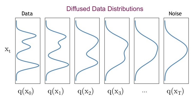
Fig. 53 Image Source: https://cvpr2022-tutorial-diffusion-models.github.io By incrementally adding noise in the forward process the distribution \(q(x_t)\) stepwise gets closer to a Gaussian normaldistribution.

Reverse Diffusion Process

In the reverse process the goal is to sample from \(q(x_{t-1}|x_{t})\). If this is possible, then the true sample can be reconstructed from Gaussian noise input \(x_T \sim \mathcal{N}(0,\mathbf{I})\). Unfortunately, in general \(q(x_{t-1}|x_{t}) \propto q(x_{t-1}) q(x_t|x_{t-1}))\) is intractable.

The solution is to estimate the true \(q(x_{t-1}|x_{t})\)-distribution by a distribution \(p_{\Theta}(x_{t-1}|x_{t})\), which is calculated by a neural network. If the \(\beta_t\)-values are small enough, \(q(x_{t-1}|x_{t})\) will be Gaussian. Hence

\[ p_{\Theta}(x_{t-1}|x_{t})=\mathcal{N}(x_{t-1};\mu_{\Theta}(x_t,t),\sigma^2 \mathbf{I}) \]

and the complete distribution of the whole process can then be calculated as follows:

\[ p_{\Theta}(x_{0:T}) = p(x_T) \prod_{t=1}^T p_{\Theta}(x_{t-1}|x_{t}) \mbox{ with } p(x_T)=\mathcal{N}(x_{T};0,\mathbf{I}). \]

After training of the U-Net, the reverse path of the Diffusion Model can be applied to generate data by passing randomly sampled noise through the learned denoising process.

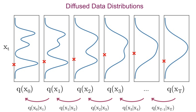
Fig. 54 Image Source: https://cvpr2022-tutorial-diffusion-models.github.io In the reverse process \(x_T\) is sampled from an isotropic Gaussian normal distribution. In each step noise is predicted and subtracted such that in the level \(t=0\) a sample from the real data distribution is available.

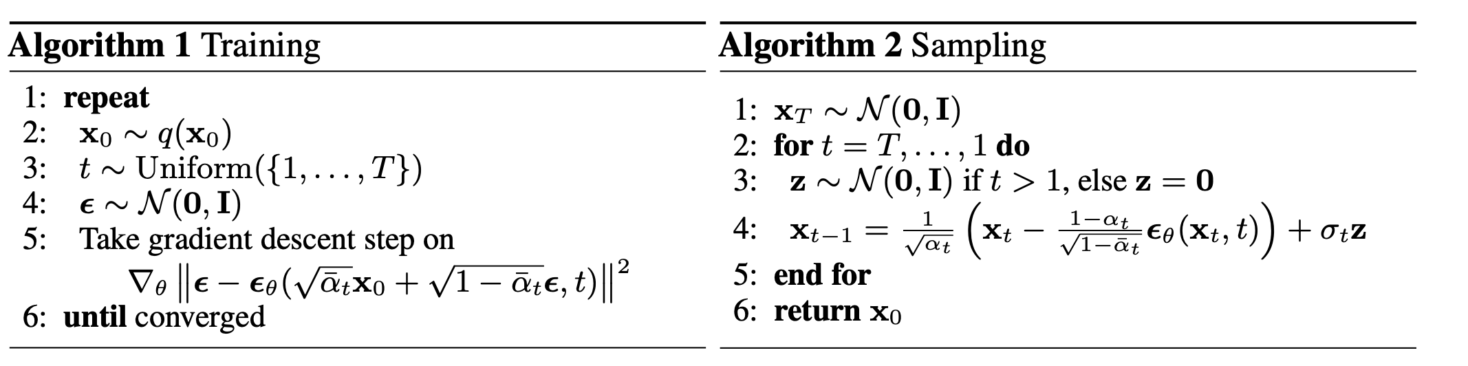
Training

Overall Idea

In the training phase the forward-process and the reverse-process are applied. In the inference phase one starts with sampling a noise-image from an isotropic Gaussian normal distribution \(\mathcal{N}(0,\mathbf{I})\). This noise sample is then passed through the reverse diffusion process. In each step of the reverse step the noise-increment between two successive image-representation is estimated by the trained neural network and subtracted from the corresponding input image \(x_t\) in order to get the less noisy representation \(x_{t-1}\).

Loss-function

The overall goal is to minimize the negative log-likelihood

\[ E \left[- \log(p_{\Theta}(x_0))\right], \]

i.e. the probability that in the reverse process the input image \(x_0\) is reconstructed shall be maximized. \(E\) is the expectation value. However, this loss function can not be applied directly because it can not be calculated in a closed form. The solution is to apply the Variational Lower Bound (https://en.wikipedia.org/wiki/Evidence_lower_bound):

\[ E \left[ - \log(p_{\Theta}(x_0)) \right] \leq E_{q} \left[ - \log(p_{\Theta}(x_0)) + D_{KL} \left(q(x_{1:T}|x_0) || p_{\Theta}(x_{1:T}|x_0)\right) \right]. \]

The evidence of this bound is clear, since the Kullback-Leibler divergence is always non-negative. The lower bound of the formula above can be rewritten in the following form:

\[ E \left[ - \log(p_{\Theta}(x_0)) \right] \leq E_{q} \left[ - \log \left(\frac{p_{\Theta}(x_{0:T}) }{q(x_{1:T}|x_0)} \right) \right] =: L_{vlb}. \]

Remark on the Variational Lower Bound!

In the inequation above the right hand side is actually an upper bound of the left hand side. However, in order to be consistent with the literature, we call it the variational lower bound. We can not minimize the left hand side directly, but indirectly by minimizing the right hand side of the inequation.

It can be shown, that the variational lower bound \(L_{vlb}\) can be expressed as a sum of KL-divergeneces:

\[ L_{vlb}=L_0 + L_1 + L_2 + \cdots + L_T, \]

with

\[\begin{split} \begin{align*} L_0 & = & -\log(p_{\Theta}(x_0 | x_1 )) \\ L_{t-1} & = & D_{KL}(q(x_{t-1} | x_t, x_0) || p_{\Theta}(x_{t-1} | x_t )) \\ L_T & = & D_{KL}(q(x_T | x_0) || p(x_T)) \\ \end{align*} \end{split}\]

For minimisation of the variational lower bound the term \(L_T\) can be ignored, because it depends only on the forward-process and \(p(x)\) is just random noise, sampled from an isotropic Gaussian.

Concerning the terms \(L_{t-1}\):

1. Due to the conditioning on \(x_0\) the \(q(x_{t-1} | x_t, x_0)\) are Gaussians

2. The \(p_{\Theta}(x_{t-1} | x_t )\) are also Gaussians:

\[ p_{\Theta}(x_{t-1}|x_{t})=\mathcal{N}(x_{t-1};\mu_{\Theta}(x_t,t),\sigma^2 \mathbf{I}) \]

Then the KL-Divergence between the two distributions is

\[ L_{t-1} \propto E_{t,x_0} \left[ || \tilde{\mu}(x_t,x_0) - \mu_{\Theta}(x_t,t)||^2 \right]. \]

with:

\[ \tilde{\mu}(x_t,x_0) = \frac{1}{\sqrt{1-\beta_t}} \left(x_t - \frac{\beta_t}{\sqrt{1-\overline{\alpha}_t}} \epsilon \right) \]

and

\[ \mu_{\Theta}(x_t,t) = \frac{1}{\sqrt{1-\beta_t}} \left(x_t - \frac{\beta_t}{\sqrt{1-\overline{\alpha}_t}} \epsilon_{\Theta}(x_t,t) \right), \]

where \(\epsilon\) is a noise sample from the isotropic Gaussian normaldistribution and \(\epsilon_{\Theta}(x_t,t)\) is the noise, predicted by the neural network at step \(t\) for given input \(x_t\).

With this parameterization \(L_{t-1}\) is

\[ L_{t-1} = E_{t,x_0,\epsilon} \left[ \lambda_t || \epsilon - \epsilon_{\Theta}(\underbrace{\sqrt{\overline{\alpha}_t}x_0 + \sqrt{1-\overline{\alpha}_t} \epsilon}_{x_t},t)||^2 \right], \]

with

\[ \lambda_t = \frac{\beta_t^2}{2 \sigma_t^2 (1-\beta_t) (1-\overline{\alpha}_t)}. \]

The authors of [HJA20] showed, that by simply setting \(\lambda_t=1\) the quality improves. They propose also that the term \(L_0\) can be neglected, yielding the simplified overall Loss-function, which is minimized during training:

\[ L_{simple} = E_{t,x_0,\epsilon} \left[ || \epsilon - \epsilon_{\Theta}(\underbrace{\sqrt{\overline{\alpha}_t}x_0 + \sqrt{1-\overline{\alpha}_t} \epsilon}_{x_t},t)||^2 \right] \]

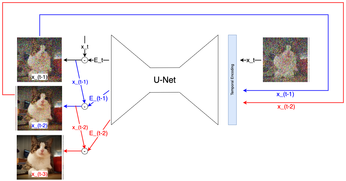
Fig. 55 Stepwise denoising in the reverse path: At time step \(t\) the image-version \(x_t\) is passed to the U-net. Given this input the U-net predicts the noise-inkrement \(\epsilon_{\Theta}(t)\) of this time-step. This noise increment is subtracted from \(x_t\). The result is the less noisier image version \(x_{t-1}\), which is passed in the next step to the input of the U-net in oder to predict \(\epsilon_{\Theta}(t-1)\).

Fig. 56 Source: [HJA20]

U-Net

U-Net is a CNN, which has been introduced in [RFB15] for biomedical image segmentation. The network consists of a contracting path and an expansive path, which gives it the u-shaped architecture. During the contraction, the spatial information is reduced while feature information is increased. The expansive pathway combines the feature and spatial information through a sequence of up-convolutions and concatenations with high-resolution features from the contracting path.

For denoising diffusion models, usually a U-Net modification, which integrates Multi-Head Attention and Residual blocks (see figures below) is applied. The U-Net is trained such that it models the reverse diffusion path.

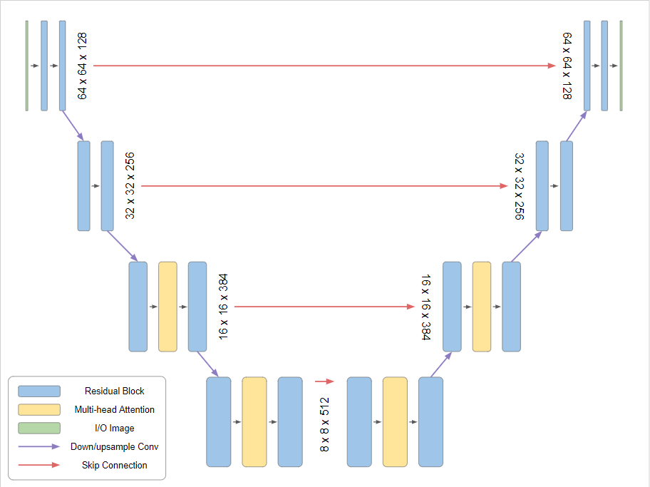
Fig. 57 Source: https://www.assemblyai.com/blog/how-imagen-actually-works/: U-Net architecture used in the reverse path of denoising diffusion models.

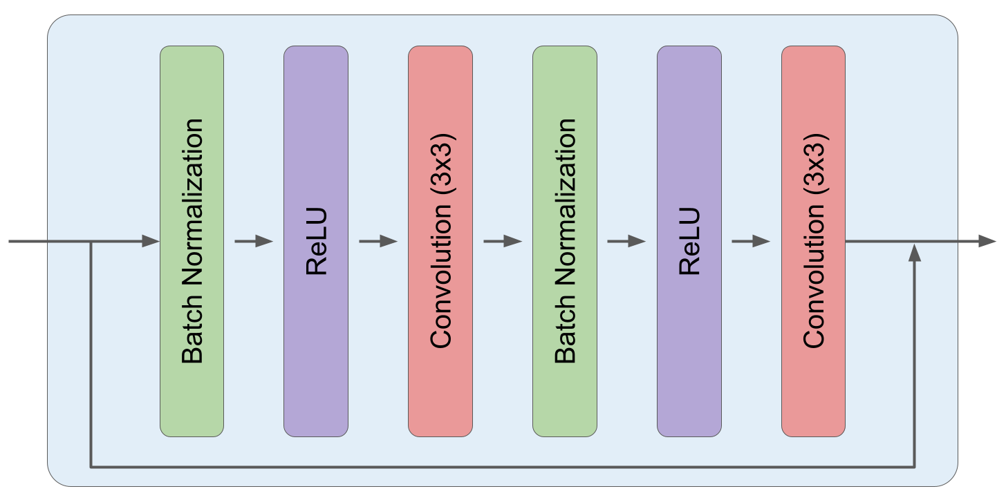
Fig. 58 Source: https://www.assemblyai.com/blog/how-imagen-actually-works/: Each residual block consists of 2 subsequences of Batch-Normalisation, Relu activation and 3x3 Convolution.