Reinforcement Learning

• Author: Johannes Maucher

• Last update: 07.01.2023

Introduction

Basic Notions

In supervised Machine learning a set of training data \(T=\lbrace (\mathbf{x}_i,r_i) \rbrace_{i=1}^N\) is given and the task is to learn a model \(y=f(\mathbf{x})\), which maps any input \(\mathbf{x}\) to the corresponding output \(y\). This type of learning is also called learning with teacher. The teacher provides the training data in the form that he labels each input \(\mathbf{x}_i\) with the corresponding output \(r_i\) and the student (the supervised ML algorithm) must learn a general mapping from input to output. This is also called inductive reasoning.

In reinforcement learning we speak of an agent (the AI), which acts in an environment. The actions \(A\) of the agent must be such that in the long-term the agent is successful in the sense that it approximates a pre-defined goal as close and as efficiently as possible. The environment is modeled by it’s state \(S\). Depending on it’s actions in the environment the agent may or may not receive a positive or negative reward \(R\) 1. Reinforcement learning is also called learning from a critic, because the agent trials different actions and sporadically receives feedback from a critic, which is regarded by the agent for future action decisions.

Reinforcement Learning refers to Sequential Decision Making. This means that we model the agents behaviour over \(time\). At each discrete time-step \(t\) the agent perceives the environment state \(S_t\) and possibly a reward \(R_t\). Based on these perceptions it must then decide for an action \(A_t\). This action influences the state of the environment and possibly triggers a reward. The new state of the environment is denoted by \(S_{t+1}\) and the new reward is denoted by \(R_{t+1}\). In the long-term the agents decision-making-process must be such, that a pre-defined target-state of the environment is approximated as efficiently as possible. The proximity of a state \(s\) to the target-state is measured by an utility function \(U(s)\).

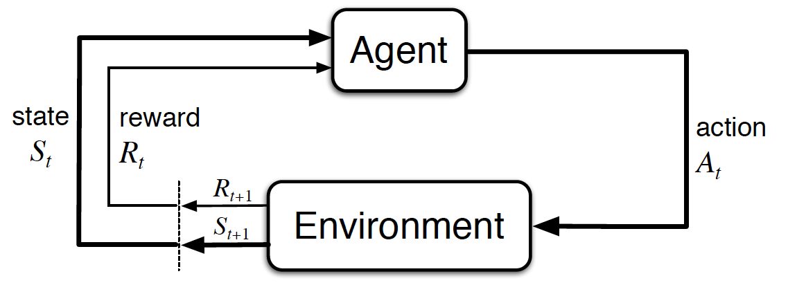
Fig. 59 Interaction of an agent with it’s environment in a Markov Decision Process (MDP). Image source: [SB18].

Examples

Board Games

Games, in particular board games like chess, checkers or Go are typical applications for reinforcement learning. The agent is the AI, which plays against a human player. The agents’s goal is to win the game. In the most simple setting it perceives a non-zero reward only at the very end of the game. This reward is positive if the AI wins, otherwise it is negative. If the AI is in turn, it first perceives the current state, which is the current board-constellation. Then it has to decide for a new action. This action modifies the state on the board. This new state is the basis for the human players action, which in turn provides a new state to the AI and so on.

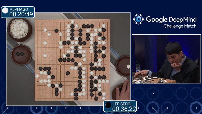
Fig. 60 Deepmind’s AlphaGo ([SHM+16]) combines Reinforcement Learning, Deep Learning and Monte Carlo Tree Search. AlphaGo was able to beat the world champion in Go, Lee Sedol, in 2016.

Non-deterministic Navigation

Navigation or similarly pathfinding can be solved by the A*-algorithm, if the environment is deterministic. This means that given the current state \(s_t\) and a selected action \(a_t\), the successive state \(s_{t+1}\) can uniquely be determined. In a non-deterministic there exist different possible successive states for a given state-action-pair. In such non-deterministic environments Reinforcemt Learning can be applied to learn an optimum policy. This policy defines for each state the action, which is best, in the sense that the expected future cumulative reward (the utility) is maximized.

In the example depicted below the task is to find the best path from the field \(Start\) to the field in the upper right corner. The possible actions of the agent are to move upwards, downwards, right or left. The environment is observable in the sense that the agent knows it’s current state. However, the environment is non-deterministic because for a known state-action-pair different successive states are possible. For this uncertainty the following probabilities are assumed to be known:

• Probability that state in the selected direction is actually reached is \(P=0.8\).

• Probability for a \(\pm 90°\) deviation is \(P=0.1\) for each.

If selected direction hits a wall, the agent remains in it’s current state. A reward of \(r_t=1\) is provided, if \(a_t\) terminates in field \((4/3)\) (the upper right corner) and a reward of \(r_t=-1\) is provided if \(a_t\) terminates in field \((4/2)\). For any other action the reward (cost) is \(r_t=-0.04\).

Fig. 61 Image source: [RN10]: Pathfinding in a non-deterministic environment

For this pathfinding scenario, the optimum policy, learned by the RL agent may look like in the picture below. The policy is defined by the arrows in the states. These arrows determine in each state the action to take in order to maximize the expected future cumulative reward.

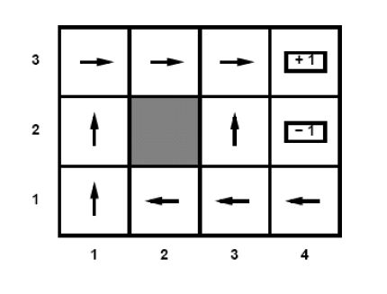
Fig. 62 Image source: [RN10]: Optimum policy learned by the RL agent

Movement of simple Robots

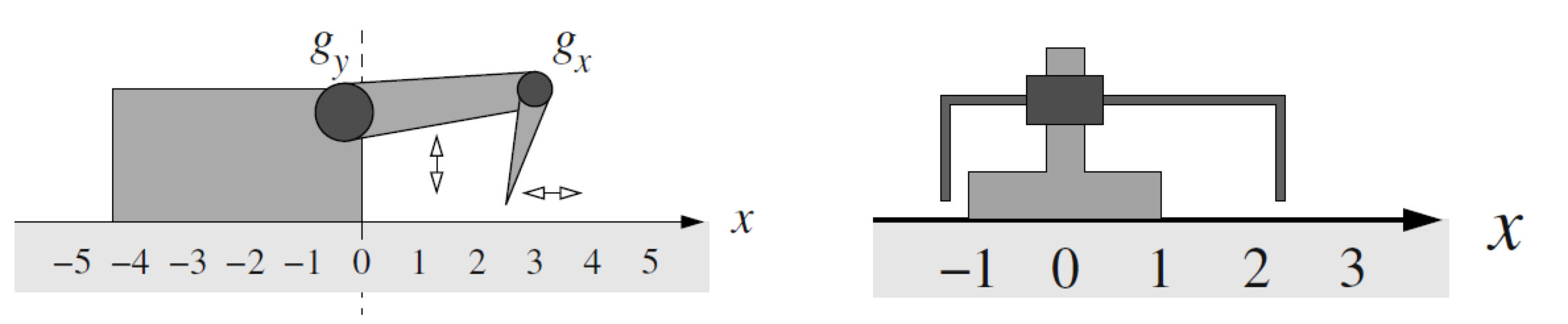
Fig. 63 Image source: [Ert09]: Two simple crawling robots. Each robot has two joints. Each joint can be in two different positions. Hence, there exists 4 different states. The robot shall learn to control the joints such that it efficiently moves from left to right. Whenever the robot moves to the right it perceives a positive reward. Movement to the left is punished with a negative reward. As can easily be verified, a movement of the robot depends not only on a single action but on a state-action-pair.

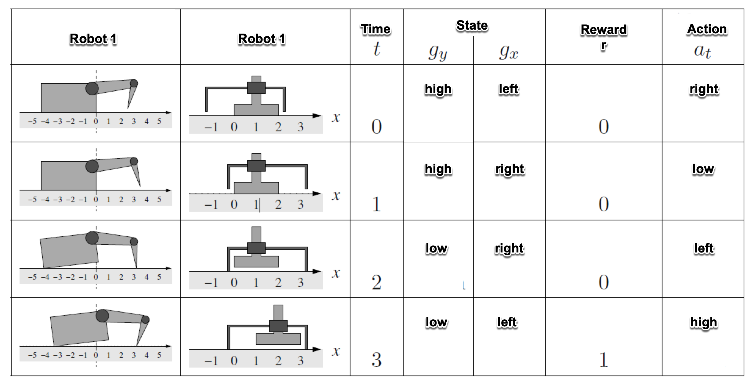
Fig. 64 Image source: [Ert09]: State \(s_t\), action \(a_t\) and reward \(r_t\) for 4 successive time-steps.

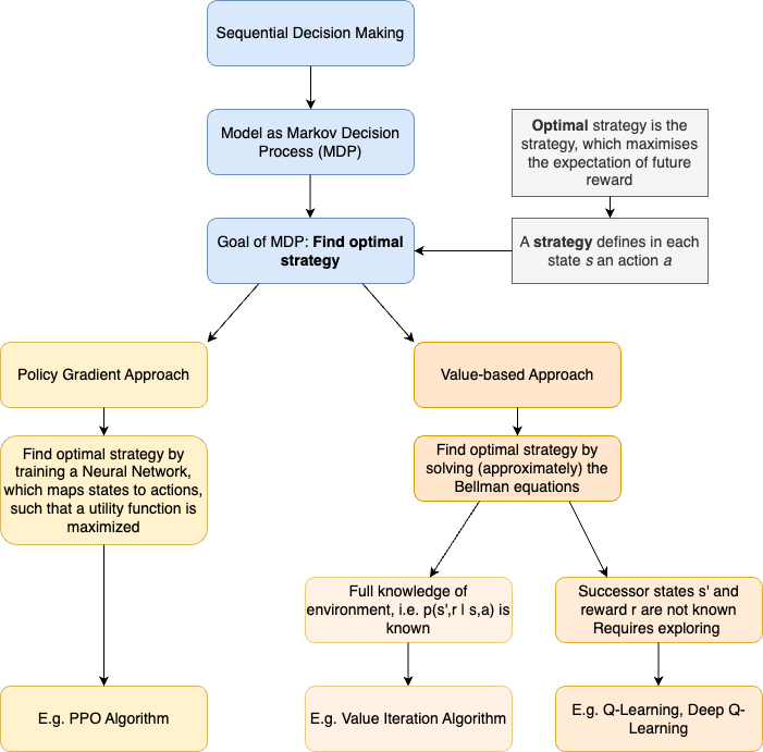
Overall Structure of this Section

The overall structure of this section is depicted below:

Markov Decision Process (MDP)

Formally, Sequential Decision Making is usually described by a Markov Decision Process (MDP). In a finite MDP the set of states \(\mathcal{S}\), the set of actions \(\mathcal{A}\) and the set of rewards \(\mathcal{R}\) is finite. For MDPs the Markovian property is assumed, which states that for each given state-action-pair, the

• probability distribution of the successive state \(S_t\) and

• the probability distribution of the successive reward \(R_t\)

depends only on the immediate preceding state and all states which lie further back need not be regarded. The function

(75)\[ p(s',r \mid s,a) = P(S_t=s',R_t=r \mid S_{t-1}=s, A_{t-1}=a) \quad \forall s`,s \in \mathcal{S}, r \in \mathcal{R} \mbox{ and } a \in \mathcal{A} \]

describes the full dynamics of the MDP. By applying the marginalisation law (see Basics of Probability Theory),

• the state-transition probability can be calculated by

(76)\[ p(s' \mid s,a) = P(S_t=s'\mid S_{t-1}=s, A_{t-1}=a) = \sum\limits_{r \in \mathcal{R}} p(s',r \mid s,a) \]

• the reward probability can be calculated by

(77)\[ p(r \mid s,a) = P(R_t=r \mid S_{t-1}=s, A_{t-1}=a) = \sum\limits_{s' \in \mathcal{S}} p(s',r \mid s,a). \]

• the expected reward can be calculated by

(78)\[ r(s,a) = \mathbb{E}(R_t \mid S_{t-1}=s, A_{t-1}=a) = \sum\limits_{r \in \mathcal{R}} p(r \mid s,a) \cdot r. \]

Markov Decision Process (MDP)

A Markov Decision Process is formally defined by

• a set of states \(\mathcal{S}\)

• a set of actions \(\mathcal{A}\)

• a state-transition-model \(p(s' \mid s,a)\) (equation (76))

• a reward-model \(p(r \mid s,a)\) (equation (77))

In a MDP the goal of an agent is to find an optimal policy \(\pi_*\), which assigns to each state \(s \in \mathcal{S}\) an action \(a \in \mathcal{A}\), such that the expected value of the cumulative sum of future received rewards is maximized. Such a policy can be determined by Reinforcement Learning.

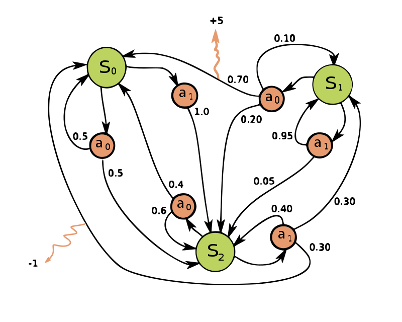
Fig. 65 Example of a simple MDP with three states (green circles) and two actions (orange circles), with two rewards (orange arrows). Image source: wikipedia.

The cumulative sum of received future rewards at time \(t\) is als called the return \(G_t\):

(79)\[ G_t= R_{t+1}+R_{t+2}+R_{t+3}+\cdots + R_{T}, \]

where \(T\) is the final time step. This formula can only be applied in the cases, where a final time step \(T\) can be defined or the entire agent-environment interaction can be partitioned into subsequences, called episodes. Whenever, such a termination can not be defined, the return can not be calculated by equation (79), because \(T=\infty\) and the return could be infinite. In order to cope with this problem a discounting rate \(\gamma\) is applied to calculate the return

(80)\[ G_t= R_{t+1}+\gamma R_{t+2}+ \gamma^2 R_{t+3}+ \cdots = \sum\limits_{k=0}^{\infty} \gamma^k R_{t+k+1}, \]

with \(0< \gamma < 1\). In this way rewards in the far future are weighted less than rewards immediately ahead and the return value will be finite. Equation (80) can easily be turned into a recursive form as follows:

(81)\[ G_t= R_{t+1}+\gamma G_{t+1} \]

Finding the Optimal Policy

As mentioned above the goal of Reinforcement Learning is to find an optimal policy \(\pi_*(a\mid s)\), which maximizes the expected return. The return has been defined in equations (79) and (80), respectively. A policy

(82)\[ \pi(a\mid s) = P(A_t=a \mid S_t=s) \]

is a function that maps to each state \(s \in \mathcal{S}\) a probability for each action \(a \in \mathcal{A}\), which is available in this state. Simply put, a strategy dictates what to do in each state.

In order to find an optimal policy Reinforcement Learning algorithms estimate Value Functions. A value function either defines

• how good it is for the agent to be in a given state. This quality is dependent of the policy \(\pi\). The state-value function for policy \(\pi\) is the expected value of return, if the agent follows strategy \(\pi\), starting from state \(s\):

(83)\[ v_{\pi}(s)= \mathbb{E}_{\pi} \left[ G_t \mid S_t=s \right] = \mathbb{E}_{\pi} \left[ \sum\limits_{k=0}^{\infty} \gamma^k R_{t+k+1} \mid S_t=s \right] \]

• how good a action \(a\) is in state \(s\). This action-value function for policy \(\pi\) measures the expected return, if the agent starts from state \(s\), takes action \(a\) in this state and then follows strategy \(\pi\):

(84)\[ q_{\pi}(s,a)= \mathbb{E}_{\pi} \left[ G_t \mid S_t=s, A_t=a \right] = \mathbb{E}_{\pi} \left[ \sum\limits_{k=0}^{\infty} \gamma^k R_{t+k+1} \mid S_t=s , A_t=a \right] \]

The task of estimating a value function is also called the prediction problem, since the value of a state or a state-action-pair is predicted. The task of finding a good policy from the previously predicted values is called control problem, since the policy defines the control of the agents actions.

How can the state-value function \(v_{\pi}\) or the action-value function \(q_{\pi}\) be estimated? One simple approach, the Monte Carlo method, is to let an agent follow policy \(\pi\). When it passes state \(s\), the future return, gained by the agent is determined (this future return is known only at the end of the episode). This is done for many times and in the end all these returns, which have been gathered whenever the agent passed state \(s\) are averaged. In the same way, the action-value function \(q_{\pi}\) can be estimated. In both cases the estimate approximates the true functions if the number of times, each state is visited, is large enough. However, in practise this Monte Carlo approach is not feasible, if the state-space, i.e. the number of different states, is large. In this case the functions can be approximated e.g. by regression. This is actually done in Deep Reinforcement Learning, where Deep Learning algorithms for regression are applied to learn good state-value- or action-value-functions from relatively few examples, gathered by the RL agent.

Bellmann Optimality Equations

As seen in equation (81) the return can be calculated recursively. Same is true for the state-value function:

(85)\[\begin{split} v_{\pi}(s) & = & \mathbb{E}_{\pi} \left[ G_t \mid S_t=s \right] \\ & = & \mathbb{E}_{\pi} \left[ R_{t+1} + \gamma G_{t+1} \mid S_t=s \right] \\ \end{split}\]

In order to calculate this expected value for a concrete state \(s\) and a concrete policy \(\pi\), one must sum up for all possible triples of \((a,s',r)\) the reward \(r\) and the discounted state-value \(v_{\pi}(s')\) of a successor state, weighted by the probability of this triple, which is given by \(\pi(a\mid s)p(s',r \mid s,a)\). This yields the Bellman equation for \(v_{\pi}\):

(86)\[\begin{split} v_{\pi}(s) & = & \sum\limits_a \pi(a\mid s) \sum\limits_{s'} \sum\limits_r p(s',r \mid s,a) \left[ r + \gamma \mathbb{E}_{\pi} \left[ G_{t+1} \mid S_{t+1}=s' \right] \right] \\ & = & \sum\limits_a \pi(a\mid s) \sum\limits_{s'} \sum\limits_r p(s',r \mid s,a) \left[ r + \gamma v_{\pi}(s') \right], \quad \forall s \in \mathcal{S} \end{split}\]

The components of this equation are visualized in the picture below. Note that this equation constitutes a relation between the value function of a state and the value-function of all successor states.

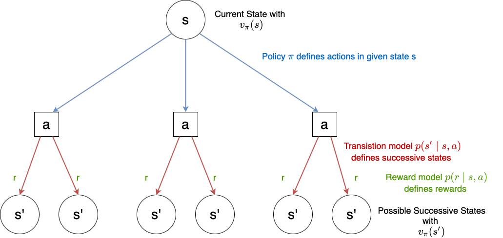
Fig. 66 Visualization of Bellman-equation (86): For a given state \(s\) and policy \(\pi\), the policy defines the probability of actions, available in \(s\). For a given state-action pair \((s,a)\) the transition model \(p(s' \mid s,a)\) defines the probability of successive states and the reward model \(p(r \mid s,a)\) defines the probability of a reward \(r\). For each of the possible succesive states \(s'\) the sum \(r + \gamma v_{\pi}(s')\) is calculated, and weighted by the probability of this \((a,s',r)\)-triple.

The state-value function of equation (86) defines an ordering of policies in the sense that one can say that policy \(\pi\) is better than policy \(\pi'\), if and only if \(v_{\pi}(s) \geq v_{\pi'}(s)\) for all states \(s \in \mathcal{S}\). Moreover, there exists at least one optimal policy \(\pi_*\), which is better than all other policies. The goal of an RL agent is to find a good approximation to this optimal policy \(\pi_*\).

The state-value function of the optimal strategy is denoted by \(v_*(s)\) and defined by:

(87)\[ v_*(s) = \max\limits_{\pi} v_{\pi}(s) \quad \forall s \in \mathcal{S} \]

Optimal policies also share the same optimal action-value function \(q_*\) ([SB18]), defined by:

(88)\[\begin{split} q_*(s,a) & = & \max\limits_{\pi} q_{\pi}(s,a) \quad \forall s \in \mathcal{S}, a \in \mathcal{A} \\ & = & \mathbb{E} \left[ R_{t+1} + \gamma v_{*}(S_{t+1}) \mid S_t=s, A_t=a \right]. \end{split}\]

Combining equations (86), (87) and (88) yields the so called Bellman optimality equation for \(v_*\):

(89)\[\begin{split} v_* (s) & = & \max\limits_{a \in \mathcal{A}(s)} q_{\pi_*}(s,a) \\ & = & \max\limits_{a} \mathbb{E}_{\pi_*} \left[ G_t \mid S_t = s, A_t=a \right] \\ & = & \max\limits_{a} \mathbb{E}_{\pi_*} \left[ R_{t+1} + \gamma G_{t+1} \mid S_t = s, A_t=a \right] \\ & = & \max\limits_{a} \mathbb{E} \left[ R_{t+1} + \gamma v_*(S_{t+1}) \mid S_t = s, A_t=a \right] \\ & = & \max\limits_{a} \sum\limits_{s'} \sum\limits_r p(s',r \mid s,a) \left[ r+ \gamma v_*(s') \right]. \end{split}\]

This equation can be visualized as follows:

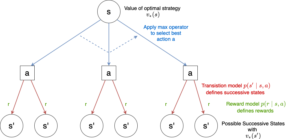
Fig. 67 Visualization of Bellman optimality equation for \(v_*\) (89).

From equation (89) the optimum policy \(\pi_*\) can easily be obtained by just taking \(argmax\) instead of \(max\). The best action in state \(s\) is

(90)\[ \pi_*(s) = \underset{a}{\operatorname{argmax}} \sum\limits_{s'} \sum\limits_r p(s',r \mid s,a) \left[ r+ \gamma v_*(s') \right]. \]

The optimum policy is definded by \(\pi_*(s)\) for all \(s \in \mathcal{S}\).

Similarly the Bellman optimality equation for \(q_*\) is:

(91)\[\begin{split} q_*(s,a) & = & \mathbb{E} \left[ R_{t+1} + \gamma \max\limits_{a'} q_*(S_{t+1},a') \mid S_t = s, A_t=a \right] \\ & = & \sum\limits_{s'} \sum\limits_r p(s',r \mid s,a) \left[ r+ \gamma \max\limits_{a'} q_*(s',a') \right]. \end{split}\]

This equation can be visualized as follows:

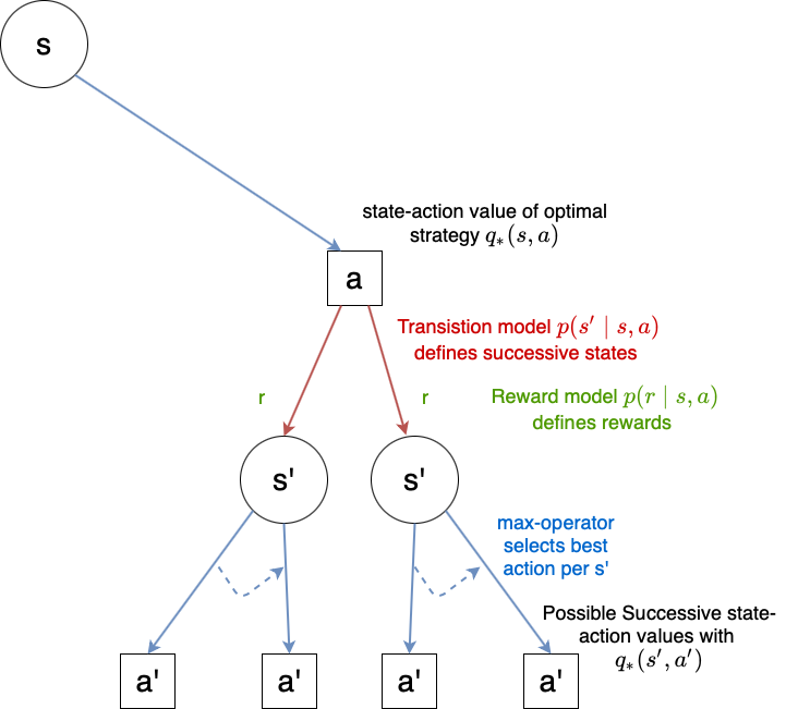
Fig. 68 Visualization of Bellman optimality equation for \(q_*\) (91).

From equation (91) the optimum policy \(\pi_*\) can easily be obtained, since in a given state the best action \(a\) is

\[ \pi_*(s) = \underset{a \in \mathcal{A}(s)}{\operatorname{argmax}} q_*(s,a). \]

Note that the Bellman optimality equations (89) and (91) are actually systems of non-linear equations, because such an equation exists for each state and each state-action-pair, respectively. In principle any method to solve systems of non-linear equations can be applied to calculate the solution. However, in practice the exact solution of these systems of equations is hardly feasible, because of the following reasons:

• the dynamics of the system, i.e. \(p(r',s' \mid s,a)\), and thus the transition-model \(p(s'\mid s,a)\) and the reward model \(p(r\mid s,a)\) must be known

• In practice systems can have many states. Then the solution of the system of non-linear equations is computational exhaustive

• the Markov property must be fulfilled

Therefore in practise methods, which approximately solve the Bellman optimality equations are applied. In the sequel such approximations will be presented. We will particularly distinguish in approximations for agents with

• complete knowledge, in this case the dynamics and therefore the transition- and reward-model are known

• incomplete knowledge, where such a complete and perfect knowledge of the environment is not available.

Dynamic Programming (DP) in the case of complete knowledge

In this section we assume complete knowledge, i.e. the environment is perfectly and completely known in terms of a finite MDP. Methods, which can be applied to calculate optimal strategies under these conditions are summarized under the term Dynamic Programming. Algorithms of this type apply utility functions such as the Bellman optimality function for \(v_*\) (89) and \(q_*\), respectively. They calculate approximations of these optimality functions by an iterative update-process. Below two famous DP algorithms, policy iteration and value iteration are described. Both of them belong to the general category of Generalized Policy Iteration, since they both iteratively evaluate and improve policies.

Policy Iteration

The general approach of the DP methods presented here consists of:

• Policy Evaluation (Prediction)

• Policy Improvement (Control)

• Policy Iteration

Starting from an initial policy \(\pi_0\), the value function \(v_{\pi_0}\) of this policy is evaluated (E). Based on this evaluation the policy is improved (I). In the next iteration, the value \(v_{\pi_1}\) is evaluated for the improved policy \(\pi_1\) and this value is again applied to calculate the new policy improvement \(\pi_2\)… and so on:

(92)\[ \pi_0 \xrightarrow{E} v_{\pi_0} \xrightarrow{I} \pi_1 \xrightarrow{E} v_{\pi_1} \xrightarrow{I} \pi_2 \xrightarrow{E} v_{\pi_2} \xrightarrow{I} \cdots \xrightarrow{I} \pi_* \xrightarrow{E} v_{\pi_*} \]

Policy Evaluation is based on the Bellman equation for \(v_{\pi}\) (equation (86)) and turns this equation into an iterative update rule. In iteration \(k+1\) a new update \(v_{k+1}(s)\) is calculated from the old \(v_{k}(s')\) of the successor-states \(s'\):

(93)\[ v_{k+1}(s) = \sum\limits_a \pi(a\mid s) \sum\limits_{s'} \sum\limits_r p(s',r \mid s,a) \left[ r+ \gamma v_k(s') \right], \quad \forall s \in \mathcal{S}, \]

The initial values \(v_0\) are chosen arbitrarily.

Policy Improvement: The reason for calculating the value function for a policy is to improve the policy. In accordance to equations (89) and (90), from the previous policy \(\pi\) and the state evaluations \(v_{\pi}\), the new policy \(\pi'\) can be calculated by

(94)\[\begin{split} \pi'(s) & = & \underset{a}{\operatorname{argmax}} q_{\pi}(s,a) \\ & = & \underset{a}{\operatorname{argmax}} \mathbb{E} \left[ R_{t+1} + \gamma v_{\pi}(S_{t+1}) \mid S_t = s, A_t=a \right] \\ & = & \underset{a}{\operatorname{argmax}} \sum\limits_{s'} \sum\limits_r p(s',r \mid s,a) \left[ r+ \gamma v_{\pi}(s') \right]. \end{split}\]

Putting policy-evaluation and -improvement into an iterative process yields the following algorithm:

Policy Iteration for estimating approximate \(\pi_*\)

1. Define value for evaluation-termination \(\epsilon\) (small positive number)

2. Initialize \(V(s) \in \mathbb{R} \mbox{ and } \pi(s) \in A(s) \mbox{ randomly } \forall s \in \mathcal{S}\). Except terminal states (if any). Terminal states must be initialized with \(0\).

3. Policy Evaluation

   • Loop:

     • Set \(\Delta := 0\)

     • Loop over all states \(s \in \mathcal{S}\):

       • Set \(v := V(s)\)

       • Calculate new \(V(s) := \sum\limits_{s'} \sum\limits_r p(s',r \mid s,\pi(s)) \left[ r+ \gamma V(s') \right]\)

       • Set \(\Delta := \max (\Delta,\mid v-V(s) \mid)\)

     until \(\Delta < \epsilon\)

4. Policy Improvement

   • Set policy-stable\(:=true\)

   • Loop over all states \(s \in \mathcal{S}\):

     • Set old-action \(:= \pi(s)\)

     • New policy:

     \[ \pi(s) = argmax_a \sum\limits_{s'} \sum\limits_r p(s',r \mid s,a) \left[ r+ \gamma V(s') \right] \]

     • If old-action \(\neq \pi(s)\), then policy-stable \(:=false\)

   • If policy-stable, then stop and return \(V \sim v_*\) and \(\pi \sim \pi_*\); else go to 3

It can be proven, that this iterative policy-evaluation and -improvement process converges to the optimal policy.

Value Iteration

The drawback of the Policy-Iteration algorithm, as given above, is that in each iteration a specific policy must be evaluated. In this evaluation \(V(s)\) of each state \(s\) is updated in many (infinite) Loop-iterations. Only after this infinite iterations the true \(v_{\pi}(s)\) is availabe and can be applied for policy improvement. The improved policy \(\pi'\) is then applied for calculating \(v_{\pi'}(s)\) and so on.

Value iterations simplifies this process, by just calculating \(V(s)\) in only one sweep and implicitely updating the policy after only one such sweep. By implicitely updating the policy, we mean (as shown in the Value iteration algorithm), that in each iteration within the loop no explicit updated policy \(\pi\) is calculated. Instead the policy is updated implicitly by the way the values \(v_{k+1}(s)\) in iteration \(k+1\) are calculated from the old \(v_{k}(s')\) of the successor-states \(s'\):

(95)\[ v_{k+1}(s) = \max\limits_{a} \sum\limits_{s'} \sum\limits_r p(s',r \mid s,a) \left[ r+ \gamma v_k(s') \right], \quad \forall s \in \mathcal{S}. \]

In the policy-iteration-algorithm the new values \(v_{k+1}(s)\) have been calculated in dependance of the policy \(\pi\). In the value-iteration algorithm these value-updates have been calculated in dependence of the best action available in the current state.

Starting from initial random values for \(v_0\) the sequence \(\lbrace v_k \rbrace\) converges to the optimal values \(v_*\) for \(k \rightarrow \infty\), if \(\gamma < 1\). In practise the value iteration algorithm terminates, if the differences of the values \(v_{k+1}\) between one iteration and the values \(v_{k}\) of the previous iteration are below a pre-defined threshold \(\epsilon\).

Value Iteration Algorithm for estimating approximate \(\pi_*\)

• Define value for termination-test \(\epsilon\)

• Initialize \(V(s) \in \mathbb{R} \quad \forall s \in \mathcal{S}\) randomly. Except terminal states (if any). Terminal states must be initialized with \(0\).

• Loop:

  • \(\Delta := 0\)

  • Loop over all states \(s \in \mathcal{S}\):

    • Set \(v := V(s)\)

    • Set \(V(s) := \max_{a} \sum\limits_{s'} \sum\limits_r p(s',r \mid s,a) \left[ r+ \gamma V(s') \right]\)

    • Set \(\Delta := \max (\Delta,\mid v-V(s) \mid)\)

  until \(\Delta < \epsilon\)

• Output policy \(\pi \sim \pi_*\), such that

\[ \pi(s) = argmax_a \sum\limits_{s'} \sum\limits_r p(s',r \mid s,a) \left[ r+ \gamma V(s') \right] \]

Example: Value Iteration Algorithm

In this simple example a deterministic transition model and a deterministic reward model is assumed. This means that for a given state-action-pair the successor and the reward is uniquely defined. Hence, for a given condition \((s,a)\) the probability \(p(s',r \mid s,a) = 1\) for exactly one pair \((s',r)\) and for all other successor-reward combinations this probability is 0.

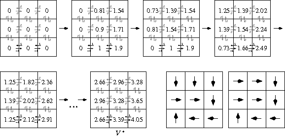
Fig. 69 The upper left grid represents the initial state of the \(3 \times 3\)-world. All states are initialized with \(v_0(s)=0\). The reward-values are assigned to the arrows. Only actions within the lower row of the world have non-negative rewards (\(-1\) for right and \(+1\) for left). The discounting-rate is assumed to be \(\gamma = 0.9\). In each iteration the states are looped through from the lower left to the upper right grid-cell. The last iteration is marked by \(V^*\). The two plots in the right bottom line are derived optimal strategies.

Fig. 70 Calculation of optimal strategy from optimal values in \(V^*\). Field \((2,3)\) is the field in the second column, third row (counted from the origin in the upper left corner). Image source: [Ert09]

Without Knowledge of the Environment

In the previous section we assumed, that complete and perfect knowledge is available. This means that the dynamics \(p(s',r \mid s,a)\) and thus the transition model \(p(s' \mid s,a)\) and the reward model \(p(r \mid s,a)\) are known. Now, we consider the case this knowledge is not available. This means that for a given state-action-pair

• the possible successive states \(s'\) and their probability distribution are not known

• the possible rewards \(r\) and their probability distribution are not known

The initially not available knowledge must be learned by the agent from experience. This experience is gathered either by the agent’s interaction with the real environment or it is gathered in a simulation. In many cases learning by interaction with the real world is not feasible, because a sufficiently frequent visit of all states or all state-action pairs, required to learn stable statistics, is not possible.

A basic concept for agents interacting with environments without perfect knowledge is:

1. In a given state \(s\) the agent somehow selects and executes an available action \(a\)

2. Only after executing the action the agents perceives the reward \(r \mid s,a\) and the successive state \(s' \mid s,a\).

The approaches described below, Monte Carlo and Temporal Difference, both can be considered as Generalized Policy Iteration, as sketched in (92).

Monte Carlo (MC) Methods

In this context we refer by Monte Carlo to methods, based on averaging complete returns over random samples (return as defined in equations (79) and (80), respectively). In contrast to MC-methods, TD-learning methods, which are described in the next subsection, learn from partial returns.

Estimation of State Value Function

As in the previous sections, the value of a state \(V(s)\) is the expected return, which is defined to be the expected cumulative future discounted reward, starting from this state \(s\). In order to estimate this value from experience, an obvious approach is to just generate many random finite walks (episods) of the agent. Whenever a given state \(s\) is visited, the return for this state is available at the end of the episode. The expected return, i.e. the value of this state, is then just the average of all returns gathered over all episodes for this state.

First-visit MC prediction for estimating state-values \(V\) of policy \(\pi\)

1. Input: Policy \(\pi\) to be evaluated

2. Initialize

   • \(V(s) \in \mathbb{R} \quad \forall s \in \mathcal{S}\) randomly.

   • For each \(s \in \mathcal{S}\): Allocate an empty list Returns(s)

3. Loop forever (for each episode):

   • Generate an episode following \(\pi\): \(S_0, A_0, R_1,S_1, A_1, R_2, \ldots, S_{T-1}, A_{T-1}, R_T\)

   • Set return \(G := 0\)

   • Loop for each step of episode, \(t=T-1,T-2,\ldots,0\):

     • Set \(G := \gamma G + R_{t+1}\)

     • Unless \(S_t\) appears in \(S_0,S_1, \ldots, S_{t-1}\):

       • Append \(G\) to \(Returns(S_t)\)

       • Set \(V(s) := average(Returns(S_t))\)

Note, the term First-visit in the name of this algorithm. As can be seen in the last unless-condition of the algorithm, only the first visit to a state \(s\) within an episode is regarded in the average return calculation for this state. There exists also an Every-visit-option of this algorithm, where all visits to \(s\) are regarded.

At this point, we can already post three differences of Monte Carlo (MC) compared to Dynamic Programming (DP):

• MC does not require knowledge of the environment in terms of a transition model and a reward model

• In MC state-evaluation (see First-visit algorithm) the estimation of a state’s value is independent of the estimated values of other (successive) states

• In MC state-evaluation (see First-visit algorithm) the computational expense of estimating the value of a single state is independent of the total number of states. This property may be of benefit, if the values of only a few states must be estimated.

Estimation of Action Value Functions

In the case of complete knowledge it was easy to derive a policy from a state value function. Since the transition model and the reward model are known, for each action the possible successive states and rewards can be determined and the best action, that can be selected to be the policy in this state. However, this is not possible if the transition- and reward model are not known. Therefore, in environments without perfect knowledge the control problem (estimating the optimal policy) is usually solved on the basis of estimating the optimal action values \(q_*\).

In principle the First-visit algorithm for state values can easily be adopted to calculate values for state-action-pairs \(q_{\pi}(s,a)\) of a policy. Instead of averaging the returns perceived in all visits of a concrete state, now on has to average the returns over all visits of a concrete state-action pair. However, the problem with such an adoption would be, that many state-action pairs would never be visited. For example if \(\pi\) is a deterministic policy, than for a given state \(s\) only one action pair \((s,a)\) will be visited. For all other actions, available in this state, no state-action values can be calculated. Note that the purpose of action-values is to gradually improve policies and if many state-actions pairs are never visited no policy-improvements can be found. In order to solve this problem it must be ensured, that all state-action-pairs can be visited, i.e. that for a given state \(s\), all actions \(a \in \mathcal{A}(s)\) have a non-zero probability to be visited. This is achieved by letting the agent to explore. The following two approaches of exploring will be condiered in the sequel:

• Exploring Starts (ES): Let each episode start in a state-action-pair and each possible state-action-pair has a non-zero probability to be selected as such a start-pair. With this approach an infinite number of episodes is required in order to guarantee, that each state-action-pair is visited sufficiently often, such that the real \(q_{\pi_k}\) is calculated for arbitrary \(\pi_k\).

• Allow only stochacstic policies for which each possible state-action pair has non-zero probability to be visited.

Monte Carlo Control

In order to find good policies the generalized concept of iteratively executing policy evaluation and policy improvement (GPI) is adopted from (92):

(96)\[ \pi_0 \xrightarrow{E} q_{\pi_0} \xrightarrow{I} \pi_1 \xrightarrow{E} q_{\pi_1} \xrightarrow{I} \pi_2 \xrightarrow{E} q_{\pi_2} \xrightarrow{I} \cdots \xrightarrow{I} \pi_* \xrightarrow{E} q_{\pi_*} \]

Policy Evaluation (E) can be done by adopting the MC First-visit algorithm to state-action-pairs \((s,a)\). If the number of episodes is infinite and the Exploring Starts (ES) approach, as defined above, is implemented, the algorithms finds the true state-action-values \(q_{\pi}\) for all arbitrary \(\pi\).

From this state-action-values \(q_{\pi}\) the policy can easily be improved (I) by:

\[ \pi(s) = \underset{a}{\operatorname{argmax}} q(s,a). \]

The drawback of this concept is the fact that an infinite number of episodes is required in the policy evaluation step in order to calculate \(q_{\pi}\). However, this problem can be solved by the same approach, which already have been applied above, where the evolution from the Policy-iteration algorithm to the Value iteration algorithm has been presented: In value-iterartion the policy is evaluated in only one sweep before it is implicitely improved. The improved policy is applied in the next iteration …and so on. Applying this idea to the Monte Carlo Policy iteration yields the algorithm below:

Monte Carlo ES (Exploring Starts) for estimating optimal policy \(\pi_*\)

1. Initialize

   • arbitrary \(\pi(s) \in \mathcal{A}(s) \quad \forall s \in \mathcal{S}\)

   • arbitrary \(Q(s,a) \quad \forall s \in \mathcal{S} \quad \forall a \in \mathcal{A}(s)\).

   • For each pair \((s,a)\): Allocate an empty list Returns((s,a))

2. Loop forever (for each episode):

   • Choose \(S_0 \in \mathcal{S}, \quad A_0 \in \mathcal{A}(S_0)\) randomly, such that all pairs have non-zero probability.

   • Generate an episode from \(S_0,A_0\) following \(\pi\): \(S_0, A_0, R_1,S_1, A_1, R_2, \ldots, S_{T-1}, A_{T-1}, R_T\)

   • Set return \(G := 0\)

   • Loop for each step of episode, \(t=T-1,T-2,\ldots,0\):

     • Set \(G := \gamma G + R_{t+1}\)

     • Unless \((S_t,A_t)\) appears in \((S_0,A_0),(S_1,A_1) \ldots, (S_{t-1},A_{t-1})\):

       • Append \(G\) to \(Returns((S_t,A_t))\)

       • Set \(Q(S_t,A_t) := average(Returns((S_t,A_t)))\)

       • Set policy \(\pi(S_t):=argmax_a Q(S_t,a)\)

The Monte Carlo ES algorithm assumes an infinite number of episodes. This is unrealistic. In practise one has to limit the number of episodes and the likelihood of finding no good policy increases with a decreasing limit of episodes. The obvious improvement is to ensure that any state-action pair can be selected with a non-zero probability, not only at the start, but during the entire episode, i.e. \(\pi(a\mid s)>0, \forall s \in \mathcal{S}, a \in \mathcal{A}\). In practise usually a small value \(\epsilon > 0\) is defined and the policy must meet the restriction

\[ \pi(a\mid s) > \frac{\epsilon}{\mid A(s) \mid}, \quad \forall s \in \mathcal{S}, a \in \mathcal{A}, \]

where \(\mid A(s) \mid\) is the number of possible actions in state \(s\). Policies, which fulfill this restriction are called \(\epsilon\)-soft policies. The most common \(\epsilon\)-soft policy is the \(\epsilon\)-greedy policy. This type chooses most of the time an action that has maximal estimated action value (Exploit), but with a small probability of \(\epsilon\) they randomly select an action from \(\mathcal{A}\) (Explore). Finding a good ratio between Exploit and Explore is called the Explore-Exploit-Dilemma. A MC control algorithm, which integrates a simple Explore-Exploit scheme is given below:

On-policy first-visit MC control for estimating policy \(\pi_*\)

1. Choose parmater \(\epsilon>0\)

2. Initialize

   • arbitrary \(\epsilon\)-soft policy \(\pi\)

   • arbitrary \(Q(s,a) \quad \forall s \in \mathcal{S} \quad \forall a \in \mathcal{A}(s)\).

   • For each pair \((s,a)\): Allocate an empty list Returns((s,a))

3. Loop forever (for each episode):

   • Generate an episode following \(\pi\): \(S_0, A_0, R_1,S_1, A_1, R_2, \ldots, S_{T-1}, A_{T-1}, R_T\)

   • Set return \(G := 0\)

   • Loop for each step of episode, \(t=T-1,T-2,\ldots,0\):

     • Set \(G := \gamma G + R_{t+1}\)

     • Unless \((S_t,A_t)\) appears in \((S_0,A_0),(S_1,A_1) \ldots, (S_{t-1},A_{t-1})\):

       • Append \(G\) to \(Returns((S_t,A_t))\)

       • Set \(Q(S_t,A_t) := average(Returns((S_t,A_t)))\)

       • Set \(A*:=argmax_a Q(S_t,a)\)

       • For all \(a \in A(S_t)\):

         • if \(a = A*\):

           • Set \(\pi(a \mid S_t) := 1 - \epsilon + \frac{\epsilon}{\mid A(S_t) \mid}\)

           else:

           • Set \(\pi(a \mid S_t) := \frac{\epsilon}{\mid A(S_t) \mid}\)

The drawback of On-policy first-visit MC control is that it can only find the best policy among the set of \(\epsilon\)-soft policies. But there may be better policies, which are not \(\epsilon\)-soft. In [SB18] this problem is stated as follows:

All learning control methods face a dilemma: They seek to learn action values conditional on subsequent optimal behavior, but they need to behave non-optimally in order to explore all actions (to find the optimal actions). How can they learn about the optimal policy while behaving according to an exploratory policy?

How can this drawback be circumvented? The answer is: by off-policy aproaches. In an off-policy algorithm the policy \(\pi\), which is iteratively evaluated and improved is not the same policy, which defines how actions are selected during the learning episodes. I.e. we have two policies:

• the target policy \(\pi\) to be optimized

• the behaviour policy \(b\), which is applied for selecting actions during the learning episodes.

By selecting the behaviour policy \(b\) to be an \(\epsilon\)-soft-policy one can ensure that all possible state-action-pairs are visited, while the target-policy \(\pi\) can be any policy without restrictions, in particular a deterministic policy. The algorithm above, On-policy first-visit MC control, is an on-policy approach. Here, behaviour during the episodes is determined by the same policy, which is evaluated and optimized.

An Off-policy MC control algorithm is given below:

Off-policy MC control for estimating policy \(\pi_*\)

1. Initialize \(\forall s \in \mathcal{S} \quad \forall a \in \mathcal{A}(s)\)

   • arbitrary \(Q(s,a) \in \mathbb{R}\).

   • \(C(s,a)=0\)

   • Policy \(\pi(s)=argmax_a Q(s,a)\)

2. Loop forever (for each episode):

   • Set \(b\) to be any \(\epsilon\)-soft policy

   • Generate an episode following \(b\): \(S_0, A_0, R_1,S_1, A_1, R_2, \ldots, S_{T-1}, A_{T-1}, R_T\)

   • Set return \(G := 0\)

   • Set \(W:=1\)

   • Loop for each step of episode, \(t=T-1,T-2,\ldots,0\):

     • Set \(G := \gamma G + R_{t+1}\)

     • Set \(C(S_t,A_t):=C(S_t,A_t)+W\)

     • Set \(Q(S_t,A_t) := Q(S_t,A_t) + \frac{W}{C(S_t,A_t)}\left[ G - Q(S_t,A_t) \right]\)

     • Set \(\pi(S_t):= argmax_a Q(S_t,a) \)

     • If \(A_t \neq \pi(S_t)\): exit inner loop. Proceed with next episode

     • Set \(W:=W \frac{1}{b(A_t \mid S_t)}\)

In this algorithm the update of the state-action values is realized by

\[ Q(S_t,A_t) := Q(S_t,A_t) + \frac{W}{C(S_t,A_t)}\left[ G - Q(S_t,A_t) \right]. \]

This is derived from the fact, that state-action-values are the expectations of the returns, as defined recursively in equation (81). However, now we have instead of the discount-factor \(\gamma\) the term \(W/C(S_t,A_t)\). The reason for this term is that the \(Q(S_t,A_t)\)-values shall be the expectation of the returns of the target policy \(\pi\), but we collected the rewards of the behaviour policy \(b\). As shown in [SB18] the term \(W/C(S_t,A_t)\) allows to map the behaviour-policy returns to the target-policy returns.

Temporal Difference (TD) Learning

If one had to identify one idea as central and novel to reinforcement learning, it would undoubtedly be temporal-difference (TD) learning. [SB18]

In Monte Carlo methods, as described above, episodes are generated, i.e. a sequence of states, actions and rewards

\[ S_0, A_0, R_1,S_1, A_1, R_2, \ldots, S_{T-1}, A_{T-1}, R_T \]

is gathered. At the end of an episode the return \(G_t\), i.e. the accumulated rewards, starting from time \(t\) up to the end of the episode, can be calculated. Only then the state-values \(V(S_t)\) or the action-state values \(Q(S_t,A_t)\) can be updated. In the case of state-values a simple MC every-visit-update method is

(97)\[ V(S_t) := V(S_t) + \alpha \left[G_t - V(S_t) \right], \]

where \(G_t\) is the actual return following time \(t\) and \(\alpha \in [0,1]\) is the step-size or learning-rate. A learning-rate of \(\alpha=0\) yields no learning (adaptation) at all, whereas \(\alpha=1\) means that the old values are not updated, but replaced. In deterministic environments \(\alpha=1\) is optimal. In stochastic environments the learning rate of reinforcement learning algorithms in general must be small, e.g. \(\alpha=0.1\) in order to guarantee convergence of the algorithm. It is also possible to decrease the learning rate with an increasing number of visits to the state, e.g.

\[ \alpha=0.1/(1+N(s)), \]

where \(N(s)\) is the number of visits to state \(s\).

In contrast to MC, TD methods need not to wait until the end of the episode to update the values. In TD-methods at time \(t\)

1. the agent in state \(S_t\) selects and executes an action \(a \in \mathcal{A}(S_t)\)

2. after executing action \(a\), the agent perceives the successor state \(S_{t+1}\) and the reward \(R_{t+1}\)

3. Then the values are updated, e.g. as follows:

(98)\[ V(S_t) := V(S_t) + \alpha \left[R_{t+1} + \gamma V(S_{t+1}) - V(S_t) \right] \]

The corresponding algorithm for policy evaluation is:

Tabular TD(0) Algorithm for estimating \(v_{\pi}\)

• Input: Policy \(\pi\) to be evaluated

• Configure: Parameter step size \(\alpha \in ]0,1]\)

• Initialize \(V(s) \in \mathbb{R} \quad \forall s \in \mathcal{S}\) randomly. Except terminal states. Terminal states must be initialized with \(0\).

• Loop for each episode:

  • Initialize S

  • Loop for each step within episode:

    • Select action \(A\) for the current state \(S\) according to policy \(\pi\)

    • Execute action \(A\) and observe reward \(R\) and successor state \(S'\)

    • Set

    \[ V(S) := V(S) + \alpha \left[R + \gamma V(S') - V(S) \right] \]

    • Set \(S:=S'\) until \(S\) is terminal state

In the update for the state-values (equation (98)) the term within the square brackets is called the TD-Error:

\[ \delta_t = R_{t+1} + \gamma V(S_{t+1}) - V(S_t). \]

It measures the difference between the estimate \(V(S_t)\) at time \(t\) and the better estimate \(R_{t+1} + \gamma V(S_{t+1})\), which can be calculated after perceiving \(R_{t+1}\) and \(S'\).

It is proven, that the TD(0) policy evaluation algorithm converges for any policy to \(v_{\pi}\), if the step-size parameter \(\alpha\) decreases. Moreover, in practice, TD-methods usually converge faster than MC methods.

In the case, that only finite experience, i.e. a limited number of episodes, is available, the most common approach is to present this experience repeatedly to the learning algorithm until it converges. In this case, from the given approximation \(V\) of the value function, the increments are calulated for each time-step of all episodes according to equation (98). Only at the end of this batch the value-function \(V\) is updated and the new increments for the entire batch are calculated w.r.t. this updated value-function and so on. This procss is called batch-updating. Under batch-updating, TD(0) converges deterministically to a single answer independent of the step-size parameter, \(\alpha\), as long as \(\alpha\) is chosen to be sufficiently small ([SB18]).

Up to now, for TD-learning, we only considered the prediction problem, in particular the calculation of the value-state function. Now, we turn to the control problem, i.e. the determination of an optimal policy.

Sarsa

As already described in the context of MC methods, in environments of incomplete knowledge, the optimal policy can not easily derived from the optimal state-value function \(v*\). Instead, the policy can be directly derived from the action-value function \(q*\). In contrast to equation (98), we now consider transitions from state-action-pair to state-action-pair and update values of such pairs:

(99)\[ Q(S_t,A_t) := Q(S_t,A_t) + \alpha \left[R_{t+1} + \gamma Q(S_{t+1},A_{t+1}) - Q(S_t,A_t) \right] \]

Since these updates require \((S_t,A_t,R_{t+1},S_{t+1},A_{t+1})\), the approach is also called Sarsa.

Sarsa: On-policy TD control for estimating \(Q \sim q_*\)

• Configure: Parameter step size \(\alpha \in ]0,1]\) and mall value \(\epsilon > 0\)

• Initialize \(Q(s,a) \in \mathbb{R} \quad \forall s \in \mathcal{S}, a \in \mathcal{A}(s)\) randomly. State-action-values of terminal states must be initialized with \(0\).

• Loop for each episode:

  • Initialize S

  • Choose \(A\) from \(S\) using policy derived from \(Q\) (e.g. \(\epsilon\)-greedy)

  • Loop for each step within episode:

    • Execute action \(A\) and observe reward \(R\) and successor state \(S'\)

    • Choose \(A'\) from \(S'\) using policy derived from \(Q\) (e.g. \(\epsilon\)-greedy)

    • Set

    \[ Q(S,A) := Q(S,A) + \alpha \left[R + \gamma Q(S',A') - Q(S,A) \right] \]

    • Set \(S:=S'\), \(A:=A'\) until \(S\) is terminal state

Q-Learning

Q-Learning is an off-policy TD reinforcement learning method. In contrast to Sarsa the learned action-value function Q directly approximates \(q_*\), the optimal action-value function, independent of the policy being followed ([SB18]).

The state-action-value update rule is

(100)\[ Q(S_t,A_t) := Q(S_t,A_t) + \alpha \left[R_{t+1} + \gamma \max\limits_a Q(S_{t+1},a) - Q(S_t,A_t) \right] \]

Q-Learning: Off-policy TD control for estimating \(\pi \sim \pi_*\)

• Configure: Parameter step size \(\alpha \in ]0,1]\) and mall value \(\epsilon > 0\)

• Initialize \(Q(s,a) \in \mathbb{R} \quad \forall s \in \mathcal{S}, a \in \mathcal{A}(s)\) randomly. State-action-values of terminal states must be initialized with \(0\).

• Loop for each episode:

  • Initialize S

  • Loop for each step within episode:

    • Choose \(A\) from \(S\) using policy derived from \(Q\) (e.g. \(\epsilon\)-greedy)

    • Execute action \(A\) and observe reward \(R\) and successor state \(S'\)

    • Set

    \[ Q(S,A) := Q(S,A) + \alpha \left[R + \gamma \max\limits_a Q(S',a) - Q(S,A) \right] \]

    • Set \(S:=S'\) until \(S\) is terminal state

Example: Q-Learning Algorithm

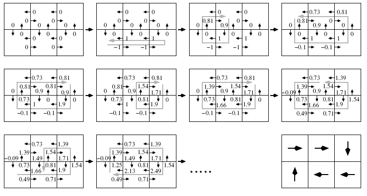
Fig. 71 Q-Learning: Updating state-action-values \(Q(s,a)\) and calculation of optimal strategy from optimal values: Initially all \(Q(s,a)\)-values are \(0\) (upper left grid). For the two states in the bottom row, for which move right is possible, the reward for action move-right is \(-1\). For the two states in the bottom row, for which move left is possible, the reward for action move-left is \(+1\). For all other state-action pairs the reward is \(0\). Image source: [Ert09]

References

• Further reading: [SB18], [RN10], [Ert09]

• RL video tutorial by deeplizard

---

1

Reinforcement is just another word for reward, hence learning from reinforcements.