Kullback-Leibler Divergence

The KL-divergence is an asymmetric statistical distance measure of how much one probability distribution P differs from a reference distribution Q. For continuous random variables the KL-divergence is calculated as follows

\[ D_{KL}(P||Q)= \int_{-\infty}^{\infty}p(x) \cdot \log\left( \frac{p(x)}{q(x)} \right) dx, \]

where \(p(x)\) and \(q(x)\) are the probability density functions of the two distributions \(P\) and \(Q\).

For discrete random variables the KL-divergence is calculated as follows

\[ D_{KL}(P||Q)= \sum\limits_{i}P(i) \cdot \log\left( \frac{P(i)}{Q(i)} \right). \]

In the discrete case the KL-divergence can only be calculated if \(Q(i) > 0\) for all \(i\) with \(P(i)>0\).

Below the KL-divergence of two Gaussian distributions is calculated and visualized.

import numpy as np
from matplotlib import pyplot as plt

Define the x-axis range:

dx=0.05
x=np.arange(-10,10,dx)

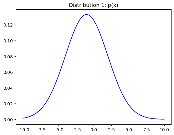
Define the first univariate Gaussian distribution:

mu1=-1
sigma1=3
dist1= 1/(sigma1 * np.sqrt(2 * np.pi)) * np.exp( - (x - mu1)**2 / (2 * sigma1**2))

fig,ax=plt.subplots()
ax.plot(x,dist1,"b")
ax.set_title("Distribution 1: p(x)")
plt.show()

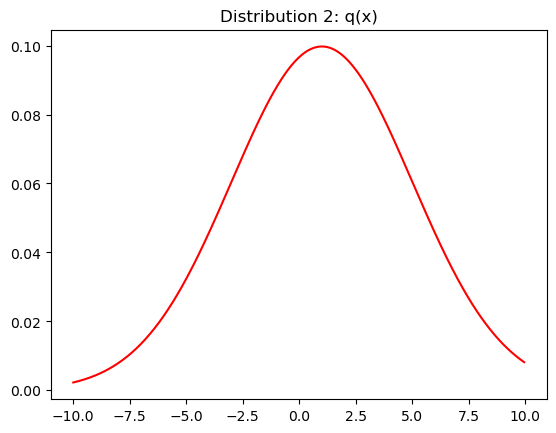
Define the second univariate Gaussian distribution:

mu2=1
sigma2=4
dist2= 1/(sigma2 * np.sqrt(2 * np.pi)) * np.exp( - (x - mu2)**2 / (2 * sigma2**2))

fig,ax=plt.subplots()
ax.plot(x,dist2,"r")
ax.set_title("Distribution 2: q(x)")
plt.show()

Kullback-Leibler- Divergence of \(p_1(x)\) with respect to \(p_2(x)\):

klsing=dist1*np.log2(dist1/dist2)
kl=np.sum(np.abs(klsing*dx))
print("Kullback-Leibler Divergence: ",kl)

Kullback-Leibler Divergence:  0.6244355861046378

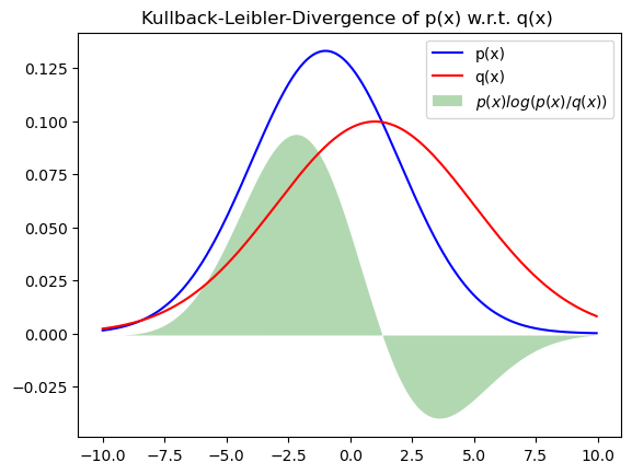
Visualization of the Kullback-Leibler Divergence. The KL-divergence is the area under the green curve:

fig,ax=plt.subplots()
ax.plot(x,dist1,"b",label="p(x)")
ax.plot(x,dist2,"r",label="q(x)")
ax.fill(x,klsing,"g",alpha=0.3,label="$p(x)log(p(x)/q(x))$")
ax.set_title("Kullback-Leibler-Divergence of p(x) w.r.t. q(x) ")
plt.legend()
plt.show()