Support Vector Machines (SVM)

Support Vector Machines (SVM) have been introduced in [CV95]. They can be applied for supervised machine learning, both for classification and regression tasks. Depending on the selected hyperparameter kernel (linear, polynomial or rbf), SVMs can learn linear or non-linear models. Other positive features of SVMs are

• many different types of functions can be learned by SVMs, i.e. they have a low bias (for non-linear kernels)

• they scale good with high-dimensional data

• only a small set of hyperparameters must be configured

• overfitting/generalisation can easily be controlled, regularisation is inherent

SVMs for Classification

SVMs learn class boundaries, which discriminate a pair of classes. In the case of non-binary classification with \(K\) classes, \(K\) class boundaries are learned. Each of which discriminates one class from all others. In any case, the learned class-boundaries are linear hyperplanes.

• In the case of a linear kernel, each learned (d-1)-hyperplane discriminates the d-dimensional space into two subspaces. \(d\) is the dimesionality of the original space, i.e. the number of components in the input-vector \(x\).

• In the case of a non-linear kernel, the original d-dimensional input data is virtually transformed into a higher-dimensional space with \(m > d\) dimensions. In this m-dimensional space training data is hopefully linear-separable. The learnd (m-1)-dimensional hyperplane linearly discriminates the m-dimensional space. But the back-transformation of this hyperplane is a non-linear discrimator in the original d-dimensional space.

The picture below sketches data, which is not linear-separable in the original 2-dimensional space. However, there exists a transformation into a 3-dimensional space, in which the given training data can be discriminated by a 2-dimensional hyperplane.

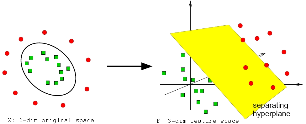
Fig. 2 Data, which is not linear-separable in the original 2-dimensional space may be linear separable in a higher dimensional space.

Another important property of SVM classifiers is that they find good class-boundaries. In order to understand what is meant by good class-boundary take a look at the picture below. The 4 subplots contain the same training-data but four different class-boundaries, each of which discriminates the given training data error-free. The question is which of these discriminantes is the best? The discriminantes in the right column are not robust, because in some regions the datapoints are quite close to the boundary. The discriminant in the top left subplot is the most robust, i.e. the one which generalizes best, because the training-data-free range around the discriminant is maximal. A SVM classifier actually finds such robust class-boundaries by maximizing the training-data-free range around the discriminant.

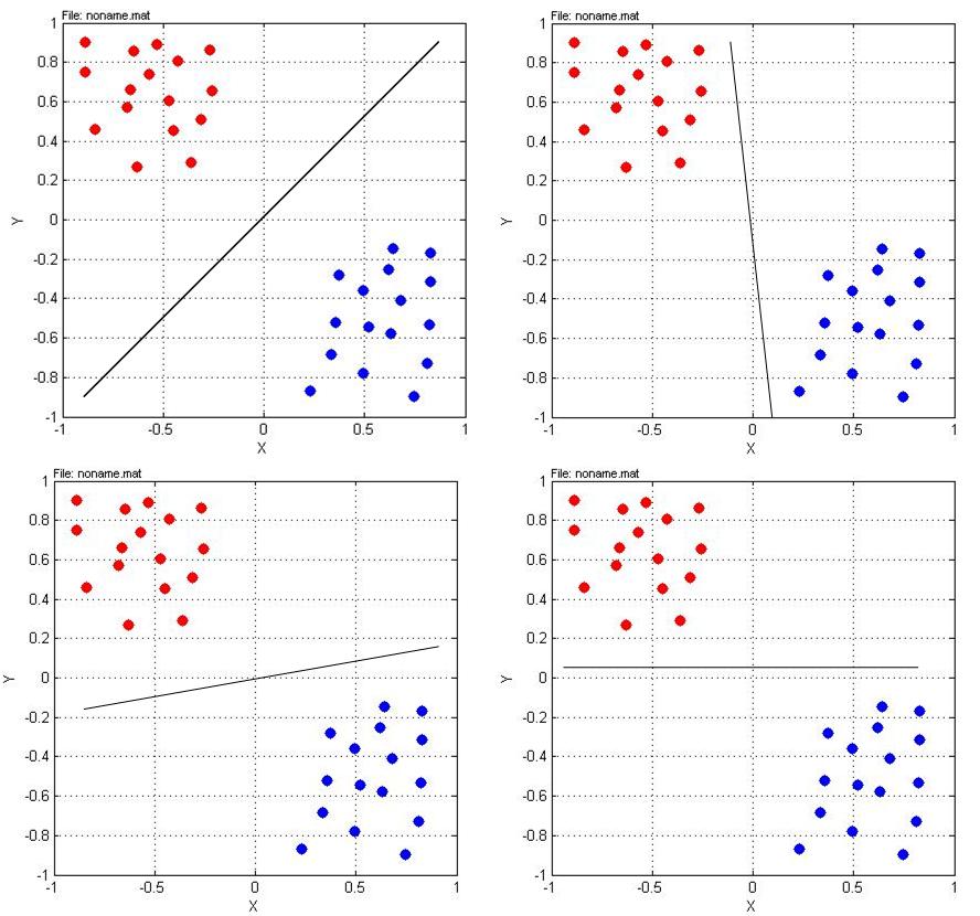
Fig. 3 The discriminant in the top left subplot is the most robust one, because it has a maximal training-data-free range around it.

Finding Robust Linear Discriminants

As mentioned above, SVM classifiers find robust discriminants in the sense that the discriminant is determined such that it not only separates the given training-data well, but also has a maximal training-data free range around it. In this subsection it is shown, how such discriminantes are learned from data. To illustrate this we apply the example depicted below. We have a set of 8 training-instances, partitioned into 2 classes. The task is to find a robust discriminant with the properties mentioned above.

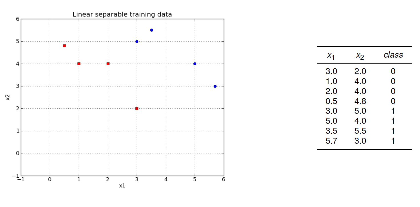
Fig. 4 Example: Learn a good discriminant from the set of 8 training-instances.

As ususal in supervised machine learning, we start from a set of \(N\) labeled training instances

\[ T=\{\mathbf{x}_p,r_p\}_{p=1}^N, \]

where \(\mathbf{x}_p\) is the p.th input-vector and \(r_p\) is the corresponding label. In the context of binary SVMs the label-values are:

• \(r_p=-1\), if \(\mathbf{x}_p \in C_1\)

• \(r_p=+1\), if \(\mathbf{x}_p \in C_2\)

The training goal is: Determine the weights \(\mathbf{w}=(w_1,\ldots,w_d)\) and \(w_0\), such that

\[\begin{split} \mathbf{w}^T \mathbf{x_p} + w_0 \geq +1 & \mbox{ for } & r_p=+1 \nonumber \\ \mathbf{w}^T \mathbf{x_p} + w_0 \leq -1 & \mbox{ for } & r_p=-1 \nonumber \label{eq:k2svmklass} \end{split}\]

This goal can equivalently be formulated by imposing the following condition

(24)\[ r_p (\mathbf{w}^T \mathbf{x_p} + w_0 ) \geq 1 \]

to be fullfilled for all training-instances. Note, that this condition defines a boundary area, rather than just a boundary line, as in other algorithms, where the condition, that must be fullfilled is:

(25)\[ r_p (\mathbf{w}^T \mathbf{x_p} + w_0 ) \geq 0 \]

The difference between the two conditions is visualized in the following picture. The plot on the left refers to condition (25). With this condition a discriminant is learned such that it separates the training-instances of the two classes. The plot on the right refers to condition (24). Here, the discriminant is learned such that the two classes are separated and the training-data-free range around the discriminant is as large as possible. The discriminant learned in this way generalizes better (less overfitting). The vectors, which ly on the region-boundary are called support vectors.

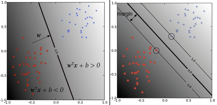
Fig. 5 Left: Other linear classification algorithms learn discriminantes, which separate the classes with as less as possible errors. Right: Discriminantes learned by SVMs have the additional property, that the training-data-free range around them is maximized.

The distance of training-instance \(\mathbf{x}_p\) to the discriminant is:

\[ \frac{|\mathbf{w}^T\mathbf{x_p}+w_0|}{||\mathbf{w}||} = \frac{r_p(\mathbf{w}^T\mathbf{x}_p+w_0)}{||\mathbf{w}||}, \quad \mbox{ where } ||\mathbf{w}|| = \sqrt{\sum\limits_{i=1}^d w_i^2} \]

The SVM training goal is to find a discrimante, i.e. parameters \(\mathbf{w}\), such that the minimum distance between a training-instance and the discriminante is maximal. Thus \(\mathbf{w}\) must be determined such that the value \(\rho\) with

\[ \frac{r_p(\mathbf{w}^T\mathbf{x}_p+w_0)}{||\mathbf{w}||}\geq \rho, \quad \forall p. \]

is maximal. Since there exists infinite many combinations of weights \(w_i\), which define the same hyperplane, one can impose an additional condition on these weights. This additional condition is

\[ \rho ||\mathbf{w}|| = 1. \]

This condition implies, that \(||\mathbf{w}||\) must be minimized in order to maximize the distance \(\rho\). We find the minimal weights and therefore the maximal \(\rho\) by minimizing

(26)\[ \frac{1}{2}||\mathbf{w}||^2 \]

under the constraints

(27)\[ r_p(\mathbf{w}^T\mathbf{x}_p+w_0)\geq 1, \quad \forall p \]

This is a standard quadratic optimisation problem with constraints. The complexity of the numeric solution of this problem is proportional to the number of dimensions in the given space. A possible optimisation method is Constraint BY Linear Approximation.

The code below shows the implementation of this example and the calculation of the discriminant from the given training data. The optimisation problem is solved by Constraint BY Linear Approximation.

from scipy.optimize import fmin_cobyla
from matplotlib import pyplot as plt
import numpy as np

#Define points and the corresponding class labels###########################
p=[[3,2],[1,4],[2,4],[0.5,4.8],[3,5],[5,4],[3.5,5.5],[5.7,3]]
c=[-1,-1,-1,-1,1,1,1,1]
#Define class which returns the constraints functions#######################
class Constraint:
    def __init__(self, points,classes):
        self.p = points
        self.c =classes
    def __len__(self):
        return len(self.p)
    def __getitem__(self, i):
        def c(x):
            return self.c[i]*(x[0]*1+x[1]*self.p[i][0]+x[2]*self.p[i][1])-1
        return c
#Define the function that shall be minimized################################
def objective(x):
    return 0.5*(x[1]**2+x[2]**2)
#Create a list of all constraints using the class defined above#############
const=Constraint(p,c)
cl=[const.__getitem__(i) for i in range(len(c))]
#Call the scipy optimization method#########################################
res = fmin_cobyla(objective,[1.0,1.0,1.0],cl)
print "Found weights of the optimal discriminant:    ",res

The figure below visualizes the discriminant, as learned in the code-cell above.

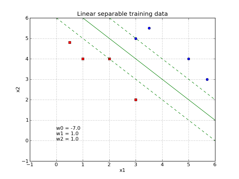
Fig. 6 The learned discriminant is characterised by having a maximum training-data free margin around it.

The complexity of the numeric solution of the quadratic minimization problem with constraints increases strongly with the dimension the underlying space. This is a problem for high-dimensional data, such as text and images. However, even if the input data contains only a moderate number of features, the space in which the optimisation problem must be solved can be extremly high-dimensional. This is because non-linear SVMs transform the given data in a high-dimensional space, where it is hopefully linear separable (as mentioned above).

This drawback of dimension-dependent complexity can be circumvented by transforming the optimisation problem into it’s dual form and solving this dual optimisation problem. The complexity of solving the dual form scales with the number of training-instances \(N\), but not with the dimensionality. Another crucial advantage of the dual form is that it allows the application of the kernel trick (see below).

Dual Form

A function \(f(x)\), such as (26), that shall be minimized w.r.t. a set of \(N\) constraints, such as (27), can always be formulated as an optimisation problems without constraints as follows:

1. reformulate all constraints to a form \(c_p(x) \geq 0\)

2. the optimisation-problem without constraints is then: Minimize

   \[ L=f(x)-\sum\limits_{p=1}^N\alpha_p \cdot c_p(x), \]

   with positive-valued Lagrange Coefficients \(\alpha_p\).

The given optimization problem defined by (26) and (27) can then be reformulated as follows: Minimize

(28)\[ L = \frac{1}{2}||\mathbf{w}||^2 \, - \, \sum\limits_{p=1}^N \alpha_p \left(r_p(\mathbf{w}^T\mathbf{x}_p+w_0)-1\right), \]

For this representation without constraints the partial derivates w.r.t. all parameters \(w_i\) are determined:

\[\begin{split} \frac{\partial L}{\partial w_i} & = & w_i - \, \sum\limits_{p=1}^N \alpha_p r_p x_{p,i} \quad \mbox{ for } i=1,\ldots,d \\ \frac{\partial L}{\partial w_0} & = & - \sum\limits_{p=1}^N \alpha_p r_p \end{split}\]

At the location of the minimum all of these partial derivatives must be 0. Setting all these equations to 0 and resolving them, such that the \(w_i\) are in isolated form on the left side of the equations yields

\[\begin{split} \mathbf{w} & = & \sum\limits_{p=1}^N \alpha_p r_p \mathbf{x}_{p} \\ 0 & = & \sum\limits_{p=1}^N \alpha_p r_p \end{split}\]

The dual form can then be obtained by inserting these equations for \(w_i\) into equation (28). This dual form is:

Maximize

(29)\[ L_d=-\frac{1}{2}\sum\limits_{p=1}^N \sum\limits_{s=1}^N \left( \alpha_p \alpha_s r_p r_s \mathbf{x}_p^T \mathbf{x}_s \right)+\sum\limits_{p=1}^N \alpha_p \]

w.r.t. the Lagrange-Coefficients \(\alpha_p\) under the restriction

(30)\[ \sum\limits_{p=1}^N \alpha_p r_p = 0 \quad \mbox{and} \quad \alpha_p \geq 0 \quad \forall p \]

This dual form can be solved by numeric algorithms for quadratic optimization. The solution reveals, that almost all of the \(N\) Lagrange-Coefficients \(\alpha_p\) are 0. The training instances \(\mathbf{x}_p\), for which \(\alpha_p>0\) are called Support Vectors.

From the \(\alpha_p>0\) and the Support Vectors, the parameters \(\mathbf{w}\) can be determined as follows:

(31)\[ \mathbf{w}=\sum\limits_{p=1}^N \alpha_p r_p \mathbf{x}_p \]

This sum depends only on the Support Vectors. Note that \(\mathbf{w}\) doesn’t contain \(w_0\). In order to determine this remaining parameter we can exploit the property of Support Vectors to lie exactly on the boundary of the region around the discriminant. This means that for all Support Vectors we have:

\[ r_p(\mathbf{w}^T\mathbf{x}_p+w_0) = 1. \]

Since we already know \(\mathbf{w}\) and we also know the Support Vectors, \(w_0\) can be calculated from this equation. Depending on which Support Vector is inserted in the equation above, the resulting \(w_0\) may vary. It is recommended to calculate for each Support Vector the corresponding \(w_0\) and choose the mean over all this values to be the final \(w_0\). Together, \(w_0\) and \(\mathbf{w}\), define the discriminant, which is called Supported Vector Machine.

As already mentioned above, in the case of non-binary classification \(K\) discriminantes must be learned. Each of which discriminates one class from all others.

Inference

Once the Support Vector Machine is trained, for a new input vector \(\mathbf{x}\) the discriminant-equation

\[ g(\mathbf{x})=\mathbf{w}^T \mathbf{x} +w_0 \]

can be calculated. If the result is \(< 0\) the input \(\mathbf{x}\) is assigned to class \(C_0\), otherwise to \(C_1\). For non-binary classification, the \(K\) discriminant-equations

\[ g_j(\mathbf{x})=\mathbf{w}_j^T \mathbf{x} +w_{0,j} \]

are evaluated, and the class for which the resulting value is maximal is selected.

Training-Data can not be separated error-free

In the entire description above, it was assumed, that the given training-data can be separated by a linear discriminant in an error-free manner. I.e. a discriminant can be found, such that all training-data of one class lies on one side of the discriminant and all training data of the other class lies on the other side of the discriminant. This assumption usually does not hold for real-world datasets. In this section SVM training is described for the general case, where training data is not linearly separable, as depicted in the image below. Again, we like to find a good discrimator for the given training-data:

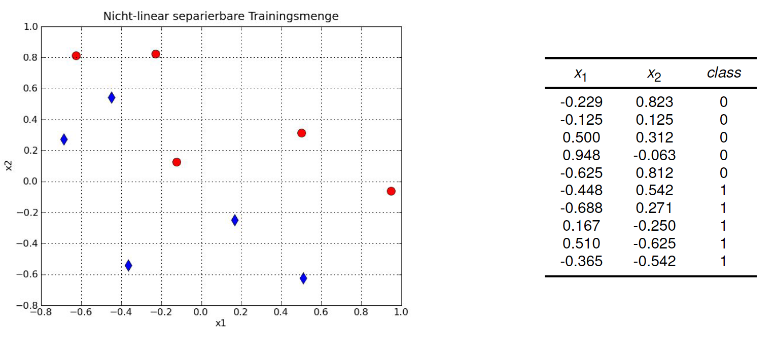
Fig. 7 Example: Learn a good linear discriminant from the set of 8 training-instances. Now training-data of the two classes is not linearly separable.

If training-data is not linear-separabel, the goal is to determine the boundary-region, which yields a minimum amount of errors on the training-data. For this to each training-instance \(\mathbf{x}_p\) an error-margin \(\zeta_p\) is assigned. The error-margin \(\zeta_p\) is

• \(\zeta_p = 0\) if \(\mathbf{x}_p\) lies on the correct side of the discriminant and outside the boundary region

• \(\zeta_p \in \left[ 0,1 \right]\), if \(\mathbf{x}_p\) lies on the correct side of the discriminant but inside the boundary region

• \(\zeta_p >1\) if \(\mathbf{x}_p\) lies on the wrong side of the discriminant

The so called Soft Error is then the sum over all error-margins

\[ \sum\limits_{p=1}^N \zeta_p \]

With this, the optimisation problem can now be reformulated to minimize

(32)\[ \min(\frac{1}{2}||\mathbf{w}||^2 + C\sum\limits_{p=1}^N \zeta_p ) \]

under the restriction

\[ r_p(\mathbf{w}^T\mathbf{x}_p+w_0)\geq 1 - \zeta_p, \quad \forall p \]

with \(\zeta_p \geq 0\)

The corresponding dual form is: Maximize

(33)\[ L_d=-\frac{1}{2}\sum\limits_{p=1}^N \sum\limits_{s=1}^N \left( \alpha_p \alpha_s r_p r_s \mathbf{x}_p^T \mathbf{x}_s \right)+\sum\limits_{p=1}^N \alpha_p \]

w.r.t. the Lagrange-Coefficients \(\alpha_p\) under the restriction

\[ \sum\limits_{p=1}^N \alpha_p r_p = 0 \quad \mbox{und} \quad 0 \leq \alpha_p \leq C \quad \forall p. \]

The parameter \(C\) in equation (32) is an important hyperparameter, which can be configured to control overfitting. A large value for \(C\) means that in the minimization process the minimization of the soft-error is more important than the minimization of the weights \(||\mathbf{w}||^2\) (i.e. the regularisation). On the other hand, a small value for \(C\) yields a discriminant with a wider margin around it and therefore a better generalizing model. This is visualized in the two plots of the figure below.

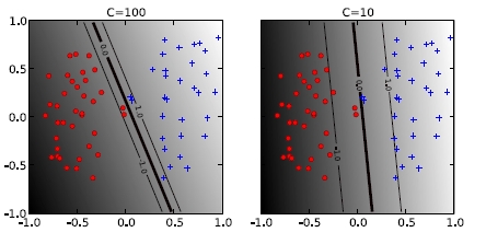
Fig. 8 Left: A high value for C implies that in the minimization process the minimization of the soft-error is more important than the maximisation of the margin around the discriminant. This yields a model, which is stronger fitted to the trainng-data than the model on the right hand side. Here a smaller value of C yields more regularisation and a thus a smaller risk of overfitting.

Again, the training instances \(\mathbf{x}_p\), for which \(\alpha_p>0\) are called Support Vectors. They lie either on the boundary of the margin around the discriminant or inside this margin.

Non-linear SVM classification

SVMs, as described in the previous subsections, find robust linear discriminants. These SVMs are said to have a linear kernel. In particular,the scalar product \(\mathbf{x}_p^T \mathbf{x}_s\) in equation (33) constitutes the linear kernel. In the sequel non-linear kernels will be introduced. The idea is to transform the inputs \(\mathbf{x}_p\) into a higher-dimensional space, where this input data is linear-separable. This idea has already been sketched in the figure above. In the figure below a concrete transformation is shown.

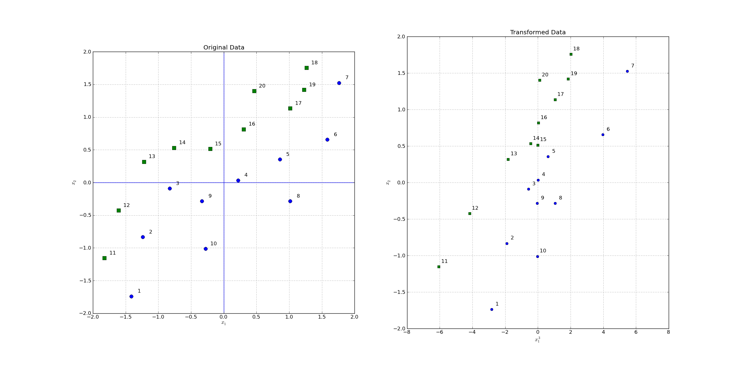
Fig. 9 Left: Original 2-dimensional space. As can be seen the two classes are not linearly separable in this space. Right: After a non-linear transformation into a new space, in this case also a 2-dimensional space, data is linearly separable. A SVM with a non-linear kernel, learns a linear discriminant into a new space, which corrsponds to a non-linear class-boundary in the original space. The transformation applied here is defined by \(z_1 = \Phi_1(x_1)=x_1^3\) and \(z_2 = \Phi_2(x_2)=x_2\)

However, as we will see later, the transformation to a higher-dimensional space need not be performed explicitely, because we can apply a kernel-trick. This kernel-trick yields the same result as the one we will get, if we would actually transform the data in a higher-dimensional space.

General Notation

• \(X\) is the d-dimensional original space in which the input-vectors \(\mathbf{x}_p\) lie.

• \(Z\) is the r-dimensional high-dimensional space (\(r>d\)), which contains the transformed input-vectors \(\mathbf{z}_p\).

• \(\Phi: X \rightarrow Z\) is the transformation from the original space \(X\) to the high-dimensional space \(Z\).

• \(\mathbf{z}_p = \Phi(\mathbf{x}_p)\) is the representation of \(\mathbf{x}_p\) in \(Z\).

Example Transformation

• Original space \(X\): \(\mathbb{R}^2\) with \(d=2\) basis-functions \(x_1\) and \(x_2\)

• High-dimensional space \(Z\): \(\mathbb{R}^6\) with \(r=6\) basis functions

\[\begin{split} z_1=\Phi_1(\mathbf{x}) & = & 1 \nonumber\\ z_2=\Phi_2(\mathbf{x}) & = & \sqrt{2}x_1 \nonumber\\ z_3=\Phi_3(\mathbf{x}) & = & \sqrt{2}x_2 \nonumber\\ z_4=\Phi_4(\mathbf{x})& = & \sqrt{2}x_1 x_2 \nonumber\\ z_5=\Phi_5(\mathbf{x}) & = & x_1^2 \nonumber\\ z_6=\Phi_6(\mathbf{x}) &=& x_2^2 \end{split}\]

The linear discriminant in the high-dimensional space \(Z\) is defined by:

(34)\[ g(\mathbf{z})=\mathbf{w}^T\mathbf{z} +w_0 \quad = \mathbf{w}^T \Phi(\mathbf{x}) +w_0 \quad = \sum\limits_{j=1}^6 w_j \Phi_j (\mathbf{x}) +w_0 \]

Kernel Trick

In the example above the number of dimensions in the high-dimensional space, in which the discriminant is determined, has been \(r=6\). In practical cases however, the dimensionality of the new space can be extremely large, such that it would be computational infeasible to transform data in this space and calculate the discriminant there. The transformation can be avoided by applying the kernel-trick, which is described here:

As in equation (31), we assume that the weights can be obtained as a weighted sum of support vectors. The only difference is that now we sum up the transformations of the support vectors:

(35)\[ \mathbf{w}= \sum\limits_{p=1}^N \alpha_p r_p \Phi(\mathbf{x}_p) \]

By inserting equation (35) into the discriminant definition (34) we obtain:

(36)\[ g(\mathbf{x})= \mathbf{w}^T \Phi(\mathbf{x}) +w_0 \quad = \sum\limits_{p=1}^N \left( \alpha_p r_p \Phi(\mathbf{x}_p)^T \Phi(\mathbf{x})\right) +w_0 \]

The kernel-trick is now to apply a non-linear kernel function \(K(\mathbf{x}_p,\mathbf{x})\), which yields the same result as the scalar-product \(\Phi(\mathbf{x}_p)^T \Phi(\mathbf{x})\) in the high-dimensional space, but can be performed in the original space.

(37)\[ g(\mathbf{x})= \sum\limits_{p=1}^N \left( \alpha_p r_p K(\mathbf{x}_p,\mathbf{x}) \right) +w_0 \]

In order to calculate this discriminant the Langrange-coefficients \(\alpha_p\) must be determined. They are obtained, as in the linear case, by maximizing

(38)\[ L_d=-\frac{1}{2}\sum\limits_{p=1}^N \sum\limits_{s=1}^N \left( \alpha_p \alpha_s r_p r_s K(\mathbf{x}_p^T, \mathbf{x}_s) \right)+\sum\limits_{p=1}^N \alpha_p \]

w.r.t. the Langrange-coefficients under the constraints

(39)\[ \sum\limits_{p=1}^N \alpha_p r_p = 0 \quad \mbox{and} \quad 0 \leq \alpha_p \leq C \quad \forall p . \]

This already describes the entire training-process for non-linear SVM classifiers. However, you may wonder how to find a suitable transformation \(\Phi\) and a corresponding kernel \(K(\mathbf{x}_p^T, \mathbf{x}_s)\)? Actually, in practical SVMs we do not take care about a concrete transformation. Instead we select a type of kernel (linear, polynomial or RBF). The selected kernel corresponds to a transformation into a higher-dimensional space, but we do not have to care about this transformation. We just need the kernel-function.

Linear Kernel

The linear kernel is just the scalar-product of the input vectors:

(40)\[ K_{lin}(\mathbf{x}_p,\mathbf{x}) = \mathbf{x}_p^T \mathbf{x} \]

By inserting this linear kernel into equation (38) we obtain equation (33). I.e. by applying the linear kernel no transform to a higher-dimensional space is performed. Instead just a linear discriminant is learned in the original space, as described in previous section.

Polynomial Kernel

Polynomial kernels are defined by

(41)\[ K_{pol}(\mathbf{x}_p,\mathbf{x}) = \left( \mathbf{x}^T\mathbf{x}_p+1\right)^q, \]

where the degree \(q\) is a hyperparameter and helps to control the complexity of the learned models. The higher the degree \(q\), the higher the dimension of the corresponding space, to which data is virtually transformed, and the higher the complexity of the learned model.

Example Polynomial kernel with degree \(d=2\)

For a degree of \(d=2\), the polynomial kernel as defined in (41) is (for a better readability we replaced \(\mathbf{x}_p\) by \(\mathbf{y}\)):

\[\begin{split} K(\mathbf{y},\mathbf{x}) & = & \left( \mathbf{x}^T\mathbf{y}+1\right)^2 \\ & = & \left( x_1y_1+x_2y_2+1 \right)^2 \\ & = & \left( 1+2x_1y_1+2x_2y_2+2x_1x_2y_1y_2+x_1^2y_1^2+x_2^2y_2^2 \right) \end{split}\]

Note that this kernel yields exactly the same result as the scalar product \(\Phi(\mathbf{y})^T \Phi(\mathbf{x})\) in the 6-dimensional space, whose dimensions are defined as in the example above.

In the image below it is shown how the different kernels (linear or polynomial) and different degrees, influence the type of discriminant. The higher the degree, the better fit to the training data but the higher the potential for overfitting.

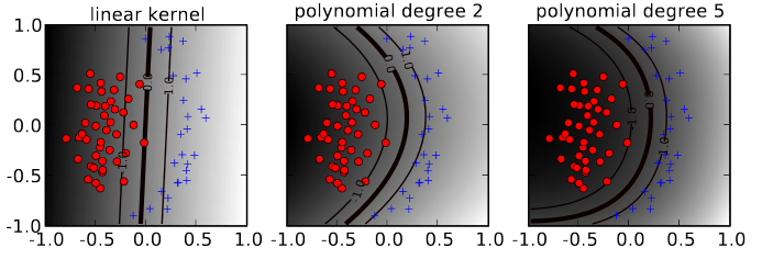
Fig. 10 Linear kernel vs. polynomial kernel of degree 2 versus polynomial kernel of degree 5. The corresponding discriminant in the original space can be complexer for increasing degree.

RBF Kernel

An important non-linear kernel type is the Radial Basis Function (RBF), which is defined as follows:

(42)\[ K_{rbf}(\mathbf{x}_p,\mathbf{x})=\exp \left[ - \gamma ||\mathbf{x}_p - \mathbf{x} ||^2 \right] \]

This function defines a spherical kernel around the support vector \(\mathbf{x}_p\). The hyperparameter \(\gamma\) determines the width of the spherical kernel. Each of the 4 plots in the image below sketches 3 RBF-kernels around different centers (support vectors) and their sum. In each of the 4 plots a different hyperparameter \(\gamma\) has been applied.

Fig. 11 1-dimensional RBFs of different degrees and different parameters \(\gamma\). In each of the 4 plots the sum of the 3 kernel-functions is plotted as a dashed-line.

In the image below for 4 different values of \(\gamma\) the discriminant learned from the given training data is shown. As can be seen, the smaller the value of \(\gamma\), the wider the spherical kernel and the smoother the sum of the kernels and the corresponding discriminant. I.e. a smaller \(\gamma\) reduces the potentential for overfitting.

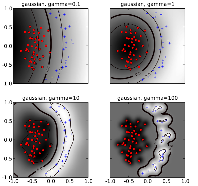
Fig. 12 1-dimensional RBFs of different degrees and different parameters \(\gamma\). In each of the 4 plots the sum of the 3 kernel-functions is plotted as a dashed-line.

SVM for Regression (SVR)

Recap Linear Regression

The supervised learning category regression has already been introduced in section Linear Regression. Recall that in linear regression during training in general the weights \(w_i \in \Theta\) are determined, which minimize the regularized loss function:

(43)\[ \mathbf{w}=argmin\left( \sum\limits_{t=1}^N [r_t-g(\mathbf{x}_t|\Theta)]^2 + \lambda \rho ||w||_1 + \frac{\lambda (1-\rho)}{2} ||w||_2^2 \right), \]

In this function, the case

• \(\lambda = 0\) refers to Ordinary Least Square without regularisation

• \(\lambda > 0 \mbox{ and } \rho=0\) refers to Ridge Regression

• \(\lambda > 0 \mbox{ and } \rho=1\) refers to Lasso Regression

• \(\lambda > 0 \mbox{ and } 0< \rho < 1\) refers to Elastic Net Regression

Optimisation Objective in SVR training

The goal of SVR training is not to find the \(g(\mathbf{x}|\Theta)\), which minimizes any variant of equation (43). Instead a \(g(\mathbf{x}|\Theta)\) has to be determined, for which the relation

(44)\[ \mid g(\mathbf{x}_t|\Theta) - r_t \mid < \epsilon \]

is true for all \((\mathbf{x}_t,r_t) \in T\). This means that all training instances must be located within a region of radius \(\epsilon\) around \(g(\mathbf{x}|\Theta)\). This region will be called the \(\epsilon\)-tube of \(g(\mathbf{x}|\Theta)\). The radius \(\epsilon\) of the tube is a hyperparameter, which is configured by the user.

In the image below a \(g(\mathbf{x}|\Theta)\), which fulfills the condition that all training instances are located within it’s \(\epsilon\)-tube is shown.

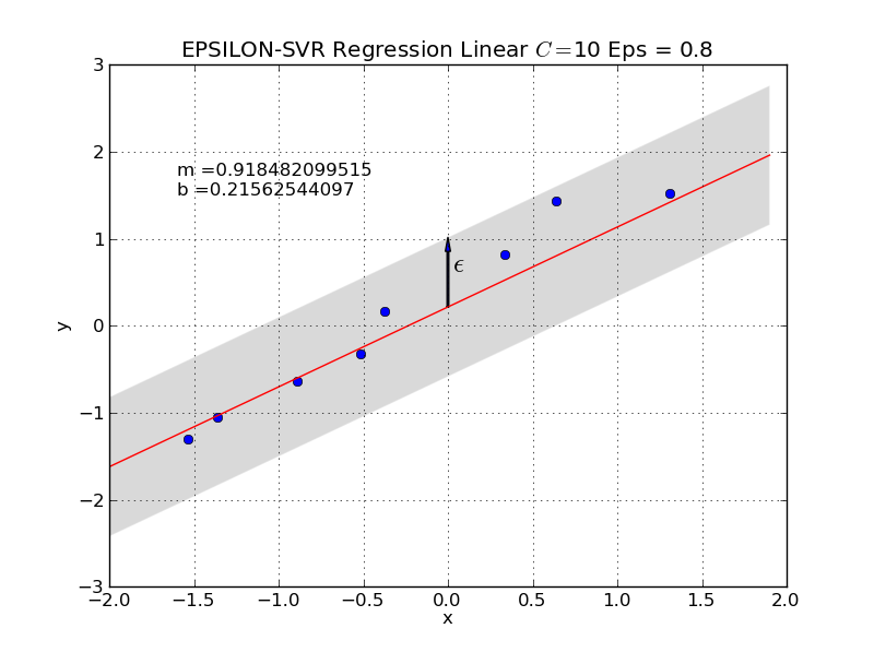
Fig. 13 For the configured \(\epsilon\) a \(g(\mathbf{x}|\Theta)\) has been determined, which fulfills condition (44) for all training elements. I.e. all training instances lie within the \(\epsilon\)-tube.

In order to find a regularized \(g(\mathbf{x}|\Theta)\), which fulfills condition (44) the following quadratic optimisation problem with constraints is solved: Find

(45)\[ \min(\frac{1}{2}||\mathbf{w}||^2) \]

such that

(46)\[ \mathbf{w}^T\mathbf{x}_t+w_0 -r_t \leq \epsilon, \quad \mbox{ or } \quad r_t-(\mathbf{w}^T\mathbf{x}_t+w_0) \leq \epsilon \quad \forall t \]

Depending on the configured value for \(\epsilon\) this optimisation problem may be not solvable. In this case a similar approach is implemented as in equation (32) for SVM classification. I.e. one accepts a soft-error for each training instance \((\mathbf{x}_t,r_t) \in T\) but tries to keep the sum over all soft-errors as small as possible.

The soft-error of a single training instance \((\mathbf{x}_t,r_t)\) is defined to be the distance between the target \(r_t\) and the boundary of the \(\epsilon\)-tube around \(g(\mathbf{x}|\Theta)\). This means that all instances, which lie within the \(\epsilon\)-tube do not contribute to the error at all!

Formally, the so called \(\epsilon\)-sensitive error function is

(47)\[\begin{split} E(T)= \sum\limits_{t=1}^N E_{\epsilon}(g(x_t)-r_t), \mbox{ where }\\ E_{\epsilon}(g(x_t)-r_t) = \left\{ \begin{array}{ll} 0 & \mbox{ if } |g(x_t)-r_t| < \epsilon \\ |g(x_t)-r_t| - \epsilon & else \\ \end{array} \right. \end{split}\]

Besides the property that deviations within the \(\epsilon\)-tube are ignored, there is another crucial difference compared to the MSE: The difference between the model’s prediction and the target contributes only linearly to the entire soft-error. This linear increase of the error, compared to the quadratic-increase of the MSE, is depicted in the image below. Because of these properties SVR regression is more robust in the presence of outliers.

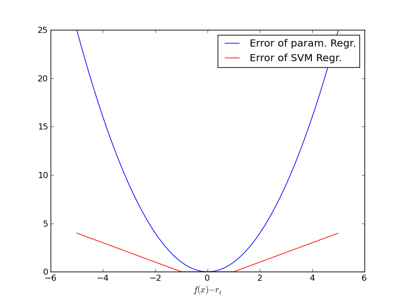
Fig. 14 Linear Increase of \(\epsilon\)-sensitive error (red) compared to quadratic increase of MSE (blue).

As already mentioned, the soft-error of a single training instance \((\mathbf{x}_t,r_t)\) is defined to be the distance between the target \(r_t\) and the boundary of the \(\epsilon\)-tube around \(g(\mathbf{x}|\Theta)\). For training instances \((\mathbf{x}_t,r_t)\) above the \(\epsilon\)-tube, the error-margin is denoted by \(\zeta_t\). For training instances \((\mathbf{x}_t,r_t)\) below the \(\epsilon\)-tube, the error-margin is denoted by \(\widehat{\zeta}_t\).

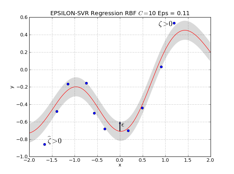
Fig. 15 Only the training instances outside the \(\epsilon\)-tube contibute to the soft-error. For instances below the tube the error margin is denoted by \(\widehat{\zeta}_t\), for instances above the tube the margin is denoted by \(\zeta_t\).

Similar as in equation (32) for SVM classification, the optimisation problem, which accepts error-margins is now:

Minimize

(48)\[ C \sum\limits_{t=1}^N(\zeta_t+\widehat{\zeta_t}) \, + \, \frac{1}{2}||\mathbf{w}||^2 \]

for \(\zeta_t \geq 0\) and \(\widehat{\zeta_t} > 0\) and

\[\begin{split} r_t - g(x_t) & \leq & \epsilon + \zeta_t \nonumber \\ g(x_t) - r_t & \leq & \epsilon + \widehat{\zeta}_t. \nonumber \\ \end{split}\]

The dual form of this optimisation problem is :

Maximize

(49)\[ L_d=-\frac{1}{2}\sum\limits_{p=1}^N \sum\limits_{s=1}^N \left( (\alpha_p-\widehat{\alpha}_p) (\alpha_s -\widehat{\alpha}_s) K(\mathbf{x}_p , \mathbf{x}_s) \right) - \epsilon \sum\limits_{p=1}^N (\alpha_p+\widehat{\alpha}_p) + \sum\limits_{p=1}^N (\alpha_p-\widehat{\alpha}_p)r_p, \]

w.r.t. the Langrange coefficients \(\alpha_p\) (corresponds to error-margin \(\zeta_p\)) and \(\widehat{\alpha}_p\) (corresponds to error-margin \(\widehat{\zeta}_p\)) under the constraints

\[\begin{split} 0 \leq \alpha_p \leq C \\ 0 \leq \widehat{\alpha}_p \leq C \\ \sum\limits_{p=1}^N (\alpha_p-\widehat{\alpha}_p) = 0 \end{split}\]

For the kernel

\[ K(\mathbf{x}_p , \mathbf{x}_s)= \Phi(\mathbf{x}_p)^T \Phi(\mathbf{x}_s) \]

in equation (49) the same options can be applied as in the classification task, e.g. linear-, polynomial- or RBF-kernel.

The result of the above optimisation are the Lagrange coefficients \(\alpha_p\) and \(\widehat{\alpha}_p\). Similar to equation (35) for SVM classification, the weights can be calculated by

(50)\[ \mathbf{w}=\sum\limits_{p=1}^N (\alpha_p-\widehat{\alpha}_p) \Phi(\mathbf{x}_p), \]

Inserting this equation for the weights into

\[ g(\mathbf{x})= \mathbf{w}^T \Phi(\mathbf{x}) +w_0 \]

yields

(51)\[ g(\mathbf{x})= \sum\limits_{p=1}^N (\alpha_p-\widehat{\alpha}_p) K(\mathbf{x},\mathbf{x}_p)+w_0 \]

The training inputs \(\mathbf{x}_p\) with \(\alpha_p \neq 0 \vee \widehat{\alpha}_p \neq 0\) are the support vectors. Only the support vectors determine the learned function. It can be shown, that all training instances \((\mathbf{x}_t,r_t)\), which lie

• within the \(\epsilon\)-tube have \(\alpha_p=\widehat{\alpha}_p=0\)

• on the upper boundary of the \(\epsilon\)-tube have \(0 < \alpha_p < C \quad \widehat{\alpha}_p = 0\)

• above the upper boundary of the \(\epsilon\)-tube have \(\alpha_p = C \quad \widehat{\alpha}_p = 0\)

• on the lower boundary of the \(\epsilon\)-tube have \(\alpha_p \quad 0 < \widehat{\alpha}_p < C\)

• below the lower boundary of the \(\epsilon\)-tube have \(\alpha_p = 0 \quad \widehat{\alpha}_p = C\)

I.e. the support vectors are all input-vectors, which do not lie within the \(\epsilon\)-tube.

In equation (51) the weight \(w_0\) is still unknown. It can be calculated for example by choosing a training instance \((\mathbf{x}_t,r_t)\) for which the corresponding Lagrange coefficient fulfills \(0 < \alpha_p < C\). This training instance lies on the upper boundary of the \(\epsilon\)-tube, i.e. \(\zeta=0\) and therefore

\[ w_0 = r_p - \epsilon - \sum\limits_{m=1}^N (\alpha_m-\widehat{\alpha}_m) K(\mathbf{x_p},\mathbf{x}_m). \]

Influence of the hyperparameters

Besides the kernel-function the most important hyperparameters of SVRs are the radius of the tube \(\epsilon\) and the parameter \(C\). As can be seen in equation (48) a higher value of \(C\) yields less importance on weight-minimmisation and therefore a stronger fit to the training data. The hyperparameter \(\epsilon\) also influences underfitting and overfitting, respectively. A large radius of the tube (large \(\epsilon\)) implies that many training-instances lie within the tube. Accordingly the number of support-vectors is small and it’s relatively easy to achieve a small overall soft-error. With wide tubes that easily cover all training elements weight-minimizsation gets easier and the chance for underfitting increases.

The influence of \(\epsilon\) and \(C\) is visualized in the images below.

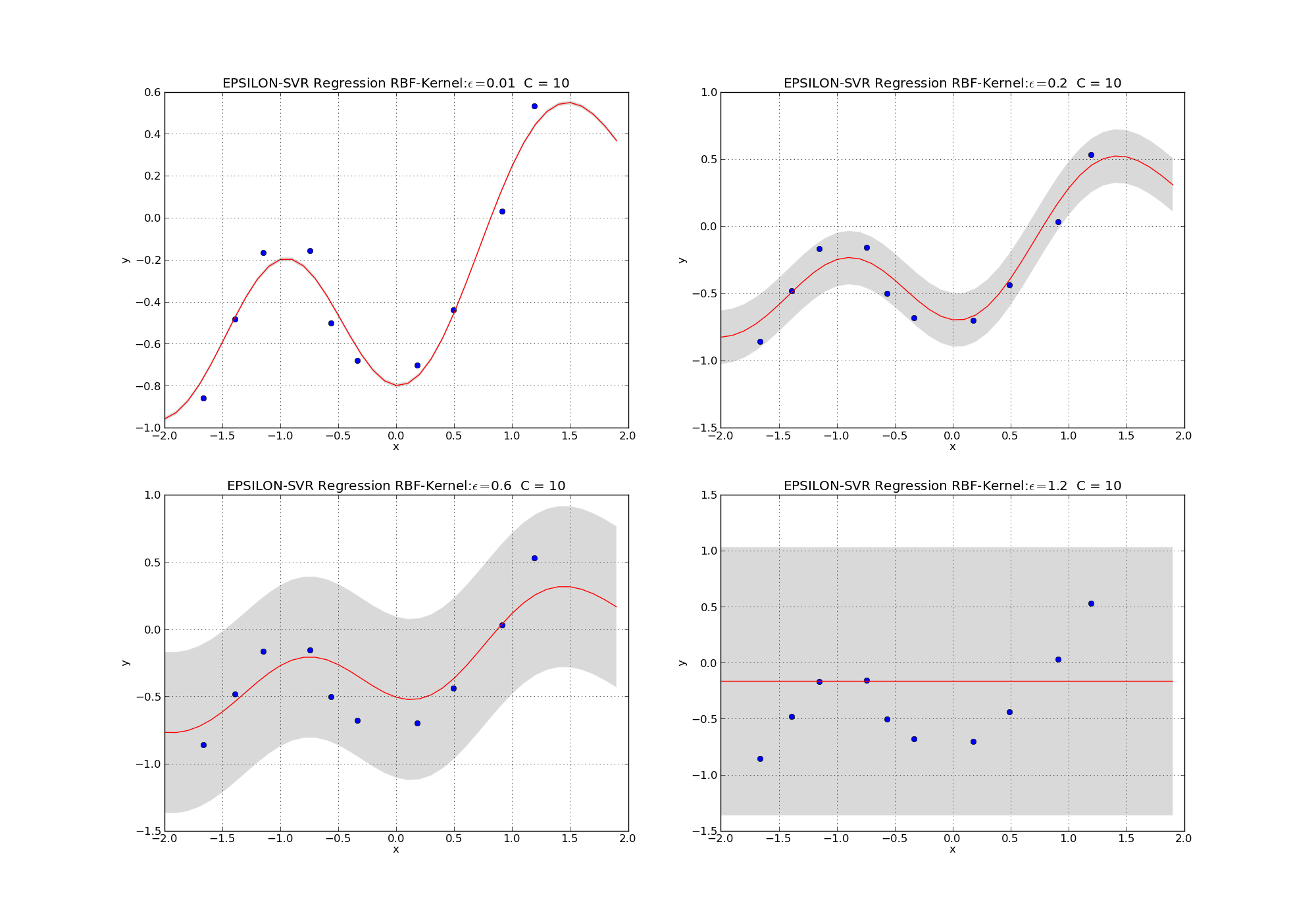
Fig. 16 Learned SVR models with RBF kernels. Parameter \(C=10\) is fixed. Parameter \(\epsilon\) increases from the upper left to the lower right plot. Smaller \(\epsilon\) increases the chance of overfitting.

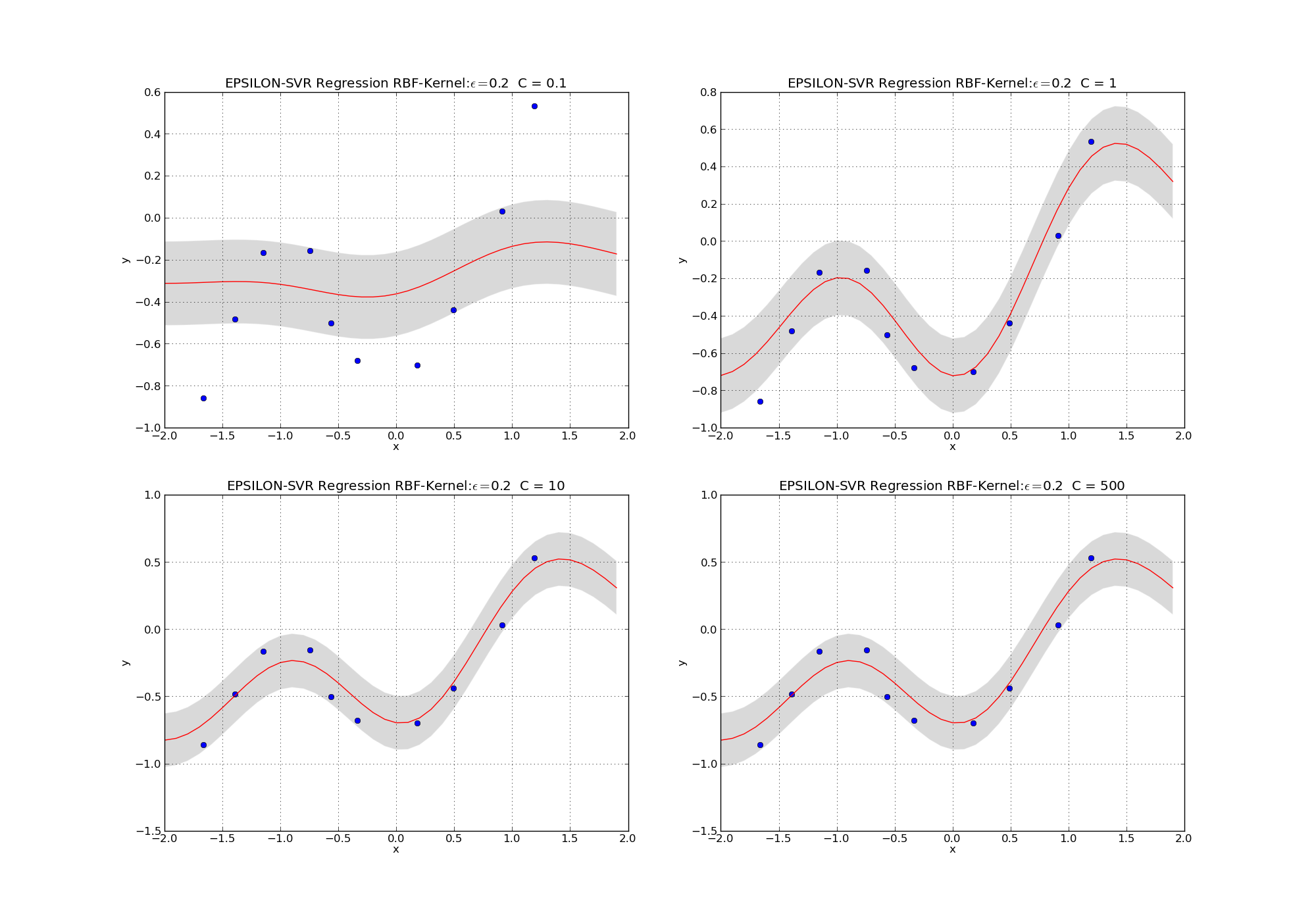
Fig. 17 Learned SVR models with RBF kernels. Parameter \(\epsilon=0.2\) is fixed. Parameter \(C\) increases from the upper left to the lower right plot. Higher \(C\) increases the chance of overfitting.

Further Reading:

• [Alp10]