Basic Concepts of Data Mining and Machine Learning
Contents
Basic Concepts of Data Mining and Machine Learning#
Author: Johannes Maucher
Last Update: 04.10.2022
Overview Data Mining Process#
The Cross-industry standard process for data mining (CRISP) proposes a common approach for realizing data mining projects:
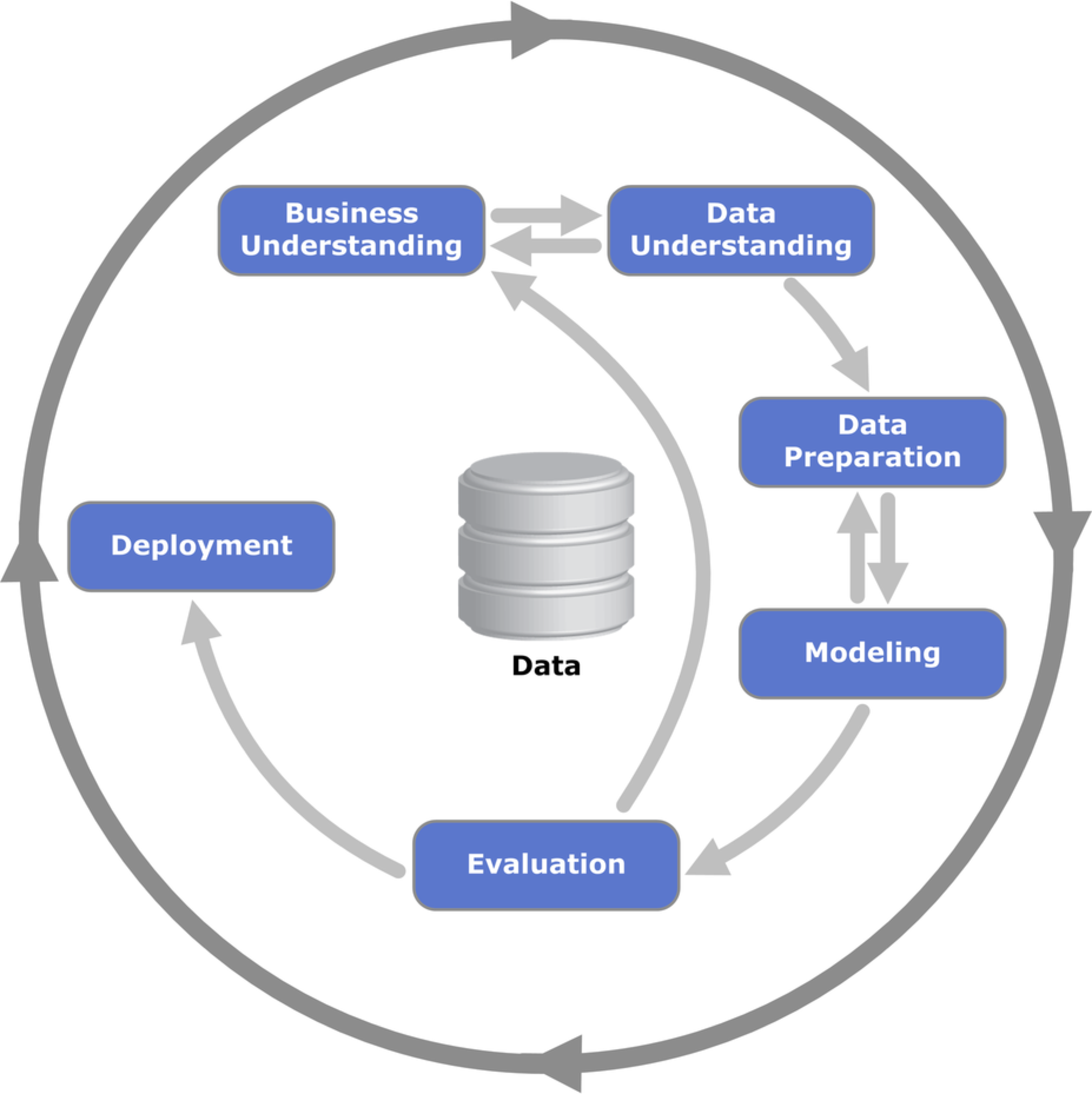
In the first phase of CRISP the overall business-case, which shall be supported by the data mining process must be clearly defined and understood. Then the goal of the data mining project itself must be defined. This includes the specification of metrics for measuring the performance of the data mining project.
In the second phase data must be gathered, accessed, understood and described. Quantitiy and qualitity of the data must be assessed on a high-level.
In the third phase data must be investigated and understood more thoroughly. Common means for understanding data are e.g. visualization and the calculation of simple statistics. Outliers must be detected and processed, sampling rates must be determined, features must be selected and eventually be transformed to other formats.
In the modelling phase various algorithms and their hyperparameters are selected and applied. Their performance on the given data is determined in the evaluation phase.
The output of the evaluation is usually fed back to the first phases (business- and data-understanding). Applying this feedback the techniques in the overall process are adapted and optimized. Usually only after several iterations of this process the evaluation yields good results and the project can be deployed.
Machine Learning: Definition, Concepts, Categories#
Machine Learning constitutes one of the 4 categories of Artificial Intelligence (AI). As shown in the image below, the other categories are Search and Planning, Knowledge and Inference and Modelling of Uncertainty.

Currently, Machine Learning is by far the most important AI category.
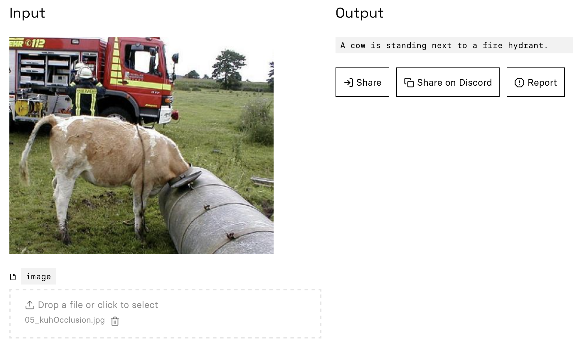
The following cartoon depicts the idea of supervised learning. A teacher provides labels for the input and a relation (model) between input and label is learned. Actually, the cartoon sketches a crucial problem of supervised Machine Learning: If we have only a small amount of training data, the learned model is overfits to a probably irrelevant feature.

Definition Machine Learning#
There is no unique definition of Machine Learning. One of the most famous definitions has been formulated in Tom Mitchell, Machine Learning:
A computer is said to learn from experience E with respect to some task T and some performance measure P , if its performance on T, as measured by P, improves with experience E.
This definition has a very pragmatic implication: At the very beginning of any Machine Learning project one should specify T, E and P! In some projects the determination of these elements is trivial, in particular the task T is usually clear. However, the determination of experience E and performance measure P can be sophisticated. Spend time to specify these elements. It will help you to understand, design and evaluate your project.
Examples: What would be T, E and P for
a spam-classifier
an intelligent search-engine, which provides individual results on queries
a recommender-system for an online-shop
Categorisation of Machine Learning Approaches#
The field of Machine Learning is usually categorized with respect to two dimensions: The first dimension is the question What shall be learned? and the second asks for How shall be learned?. The resulting 2-dimensional matrix is depicted below:

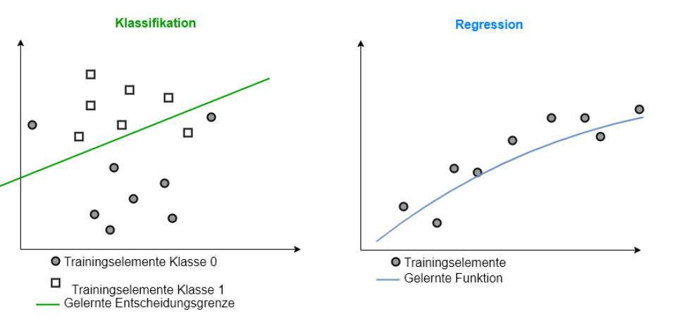
On an abstract level there exist 4 answers on the first question. One can either learn
a classifier, e.g. object recognition, spam-filter, Intrusion detection, …
a regression-model, e.g. time-series prediction, like weather- or stock-price forecasts, range-prediction for electric vehicles, estimation of product-quantities, …
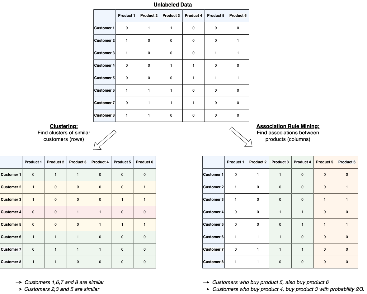
associations between instances, e.g. document clustering, customer-grouping, quantisation problems, automatic playlist-generation, ….
associations between features, e.g. market basket analysis (customer who buy cheese, also buy wine, …)
strategie, e.g. for automatic driving or games
On the 2nd dimension, which asks for How to learn?, the answers are:
supervised: This category requires a teacher who provides labels (target-values) for each training-element. For example in face-recognition the teacher most label the inputs (pictures of faces) with the name of the corresponding persons. In general labeling is expensive and labeled data is scarce.
unsupervised learning: In this case training data consists only of inputs - no teacher is required for labeling. For example pictures can be clustered, such that similar pictures are assigned to the same group.
Reinforcement learning: In this type no teacher who lables each input-instance is available. However, there is a critics-element, which provides feedback from time-to-time. For example an intelligent agent in a computer game maps each input state to a corresponding action. Only after a possibly long sequence of actions the agent gets feedback in form of an increasing/decreasing High-Score.
Supervised Learning#

Apply Learned Modell:

Unsupervised Learning#

Apply learned Model:

Associations between Instances (Clustering) and Associations between Features (Association Rule Mining):
Reinforcement Learning: Learning from Feedback#

General Scheme for Machine Learning#
In Machine Learning one distinguishes
training-phase,
validation-phase,
test-phase,
operational phase.
Training and validation are shown in the image below.
In the training phase training-data is applied to learn a general model. The model either describes the structure of the training data (in the case of unsupervised learning) or a function, which maps input-data to outputs.
Validation phase: During the training-phase the model is fitted to the training-data. However, the primal goal is not to find a model, which is maximally fitted to training data. Instead we like to learn a model, which generalizes well, i.e. it shall be good on new data, which has not been seen during training. For this a validation-data partition, which is disjoint to the training-data partition, is applied to the model. This means, that for each input of the validation-partition the learned models prediction is calculated and compared to the true output (label). In this way an error-statistic, more general: a performance-measure, can be calculated. The performance measure on the validation data is used to assess the learned model, to compare different models and to select the best trained model.
Test phase: In order to estimate the selected models performance in real life, one applies a test-data partition, which is disjoint to training-data and validation-data. The performance on the test-data tells us the accuracy we can expect in the operational mode.
Operational mode: If the performance in the preceding test phase is sufficient for our purpose, the model can be deployed to the target device. In the operational mode, the model receives new input data and has to calculate the corresponding output (class, prediction, etc.)
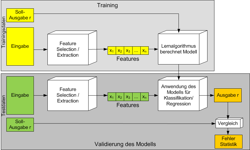
As shown in the picture above, usually the available data can not be passed directly to the machine-learning algorithm. Instead it must be processed in order to transform it to a corresponding format and to extract meaningful features. The usual formal, accepted by all machine-learning algorithms is a 2-dimensional array, whose rows are the instances (e.g. documents, images, customers, …) and whose columns are the features, which describe the instances (e.g. words, pixels, bought products, …):
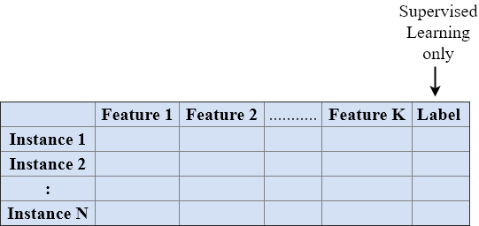
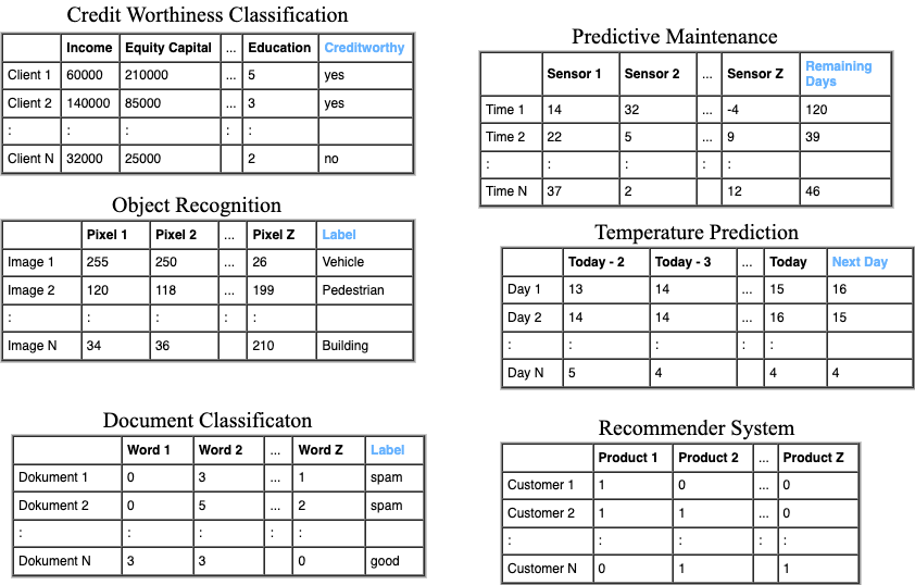
The image below depicts such a 2-dimensional array of training-data for the applications Object Recognition, Document Classification, Personality Classification, Temperature Prediction and Recommender System.
General Concept of Supervised Learning#
The general concept of supervised learning is sketched in the image below. This concept is realized by almost all algorithms for supervised machine learning, in particular all neural networks learn according to this approach. In the following description it is assumed that the ML algorithm is a Neural Network.
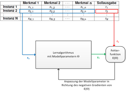
General concept of iterative supervised learning:
The network parameters \(\Theta\) are initialized randomly
Apply the input vectors \(\mathbf{x}_p\) of one or more training instances to the input of the network
Calculate the corresponding output of the network \(y=f(\mathbf{x}_p,\Theta)\)
Calculate the error between the calulated outputs \(y\) and the corresponding target labels \(r\)
Depending on the calculated errors, adjust the network weights \(\Theta\), such that in the sequel the network outputs are closer to the targets (i.e. the error decreases).
Repeat this until the calculated error is small enough.
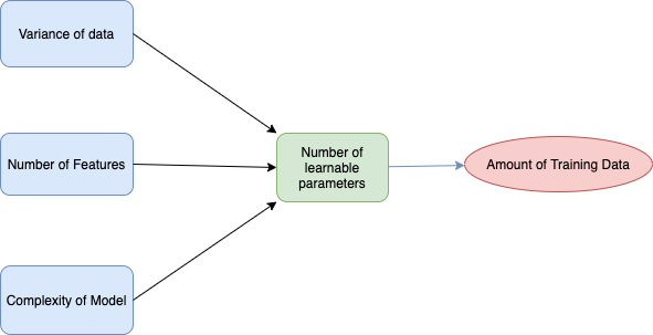
Required Amount of data (supervised learning)#
One of the crucial questions at the beginning of each ML-procect is
How much labeled data is required?
The answer is: It depends!
Unfortunately one calculate the required amount of labeled data for
training
validation
test.
However, the main factors, which influence the amount of labeled data, are known and depicted below:
Further Categories#
Even though Machine Learning showed amazing accuracy in a wide range of tasks such as object classification, machine translation and automated content generation, many experts are convinced that in order to create human-level AI new approaches to ML and AI must be invented. The current methods, in particular supervised learning, is supposed to get stuck in a suboptimum, far from human-level AI. The reason for these doubts is that supervised ML requires large amounts of labeled data and in general labeling is expensive. On the other hand a main factor of human intelligence is common sense, i.e. knowledge on general concepts such as gravity or object permanence. Human’s create common sense from their birth on, mainly by unsupervised observation of the world. It is because of this understanding of common concepts that makes our learning of specific things efficient. For example, based on the knowledge of gravity, we do not need much specific training samples in order to predict the trajectory of a stone, which is thrown away.
It is clear that supervised learning alone will not be sufficient to teach machines something like common sense, since it is impossible to label everything. Therefore, recent ML research has a strong focus on finding new methods for learning from unlabeled data. In particular concepts that exploit both, a relatively small set of labeled data and a large set of unlabeled data, are investigated. Two main categories of this type are self-supervised learning and semi-supervised learning.
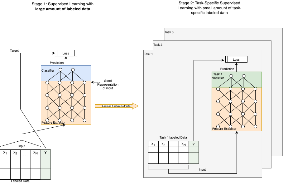
Self-Supervised Learning#
Self-supervised learning consists of 2 stages: First large amounts of unlabeled data are applied to learn a feature-extractor, which provides a good representation of the given data domain. This feature-extractor is passed to stage 2, where it can be applied for many different tasks with the same input data domain. In order to learn these task-specific models in the 2nd stage only relatively small amounts of task-specific labeled data is required. This concept is depicted in the image below. Examples are e.g. Word2Vec or transformers like BERT. In both examples unlabeled text data (e.g. the entire Wikipedia, or tons of books) are applied for pretraining. During pretraining the feature-extractor is trained such that it predicts masked words (target) from the surrounding words (input).
Self-supervised learning is only applicable, if there exist semantic relations between the elements \(x_i\) of the unlabeled data. This is true e.g. for text (words within sentences are related), images (neighbouring pixels are correlated) and video (successive frames within the video are correlated).
Semi-Supervised Learning#
Semi-supervised learning is another approach to learn models from relatively small amounts of labeled data and large amounts of unlabeled data. The trick in self-supervised learning was to apply in stage 1 a supervised-learning approach on unlabeled data. This is feasible only if there exists semantic relations between the elements of the input-data-vectors. Now, in semi-supervised learning, we do not have to impose this hard restriction on the structure of data. However, there exist other assumptions, which must be fullfilled (at least one), e.g. the
Continuity Assumption: Input-vectors, which are close to each other, likely share the same label.
Cluster Assumption: The set of all input-vectors is grouped in different clusters and vectors within the same cluster likely share the same label.
Manifold-Assumption: Input vectors lie approximately on a manifold (subspace) of much lower dimension than the input space.
Semi-supervised learning may refer to either transductive learning or inductive learning.The goal of transductive learning is to infer the correct labels for the given unlabeled data only. The goal of inductive learning is to infer the correct mapping from input data to target in general. (Source: Wikipedia).
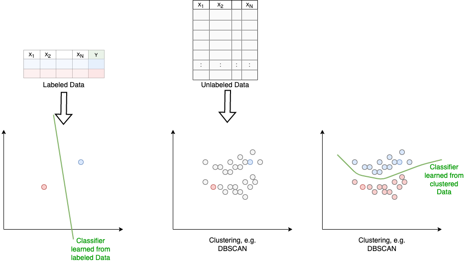
There exists many approaches for semi-supervised learning. One is to use the labeled data to learn an initial classification model. Then the unlabeled data is applied to learn better class-specific distributions, which provide better classifiers.
Supervised Pretraining#
A common and extremely efficient approach to apply deep neural networks in the case of only relatively small amounts of labeled training data is to integrate neural networks, which have been pretrained on a very large labeled dataset. Such pretrained deep neural networks can be downloaded e.g. from
As in the case of self-supervised learning, the learned feature extractor constitutes a basis, which can be adapted and fine-tuned for different tasks. Again, a relatively small amount of task-specific labeled data is required for fine-tuning.
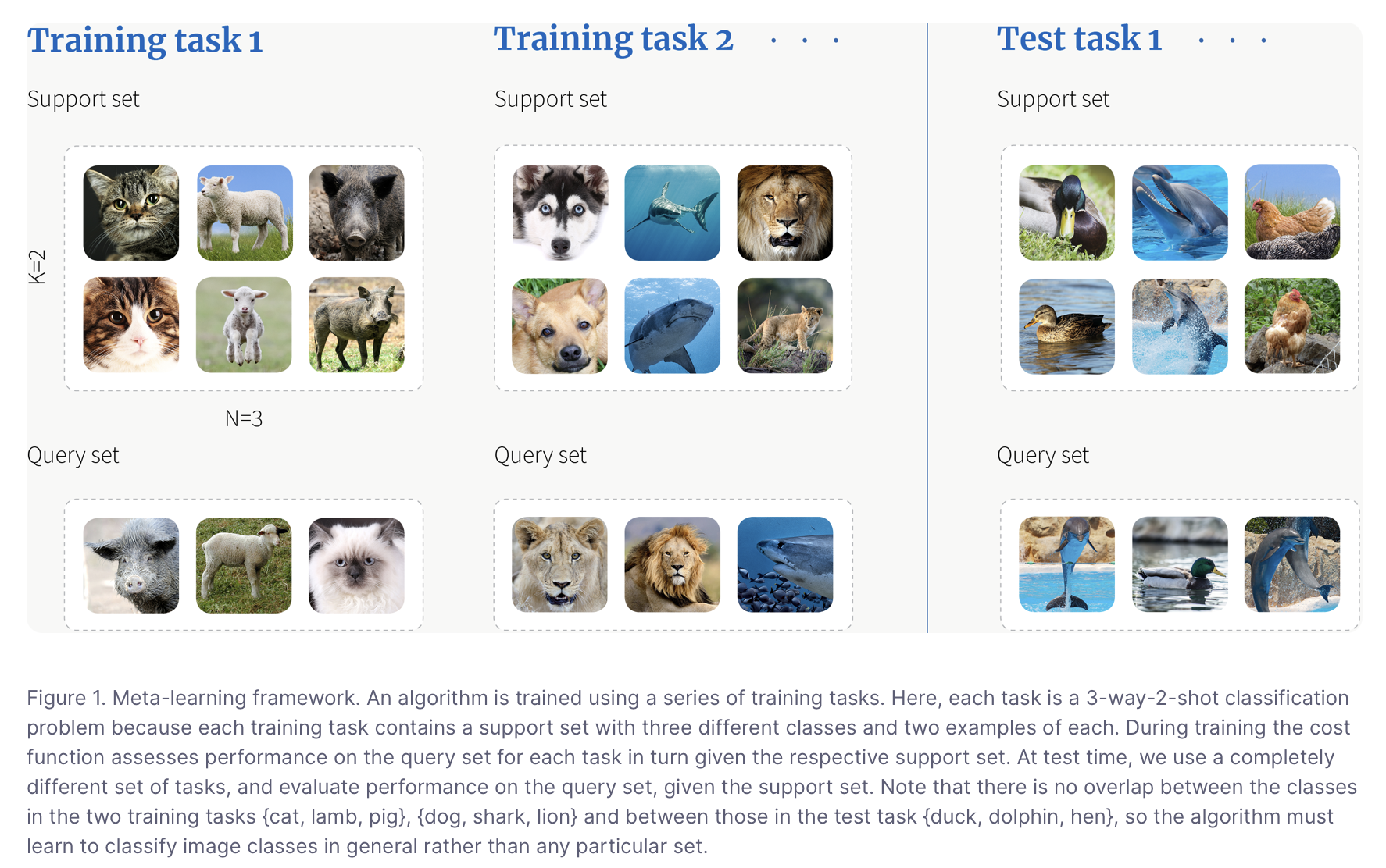
Few-Shot Learning#
The term Few-Shot-Learning refers to approaches, which provide models that can be applied for classification, even though there is only a very small amount of labeled data - too small to apply conventional ML. In the extreme case of One-Shot-Learning only one labeled training instance per class is required.
Few-Shot-Learning is often described as N-way-K shot meta learning classification. This means that for each of the \(N\) classes \(K\) labeled training instances are available. Typical numbers for \(N\) and \(K\) are 10 and 5, respectively.
As sketched in the image below (Image Source: https://www.borealisai.com), the idea of meta learning is to learn how to classify by training a network on different but similar tasks. The more similar tasks are applied to learn the network’s weight, the better it’s capability to distinguish classes in general.
A quit popular realisation of few-shot-learning is the Matching Networks approach, which has been introduced in O. Vinyals et al. The picture below describes the idea of this approach:
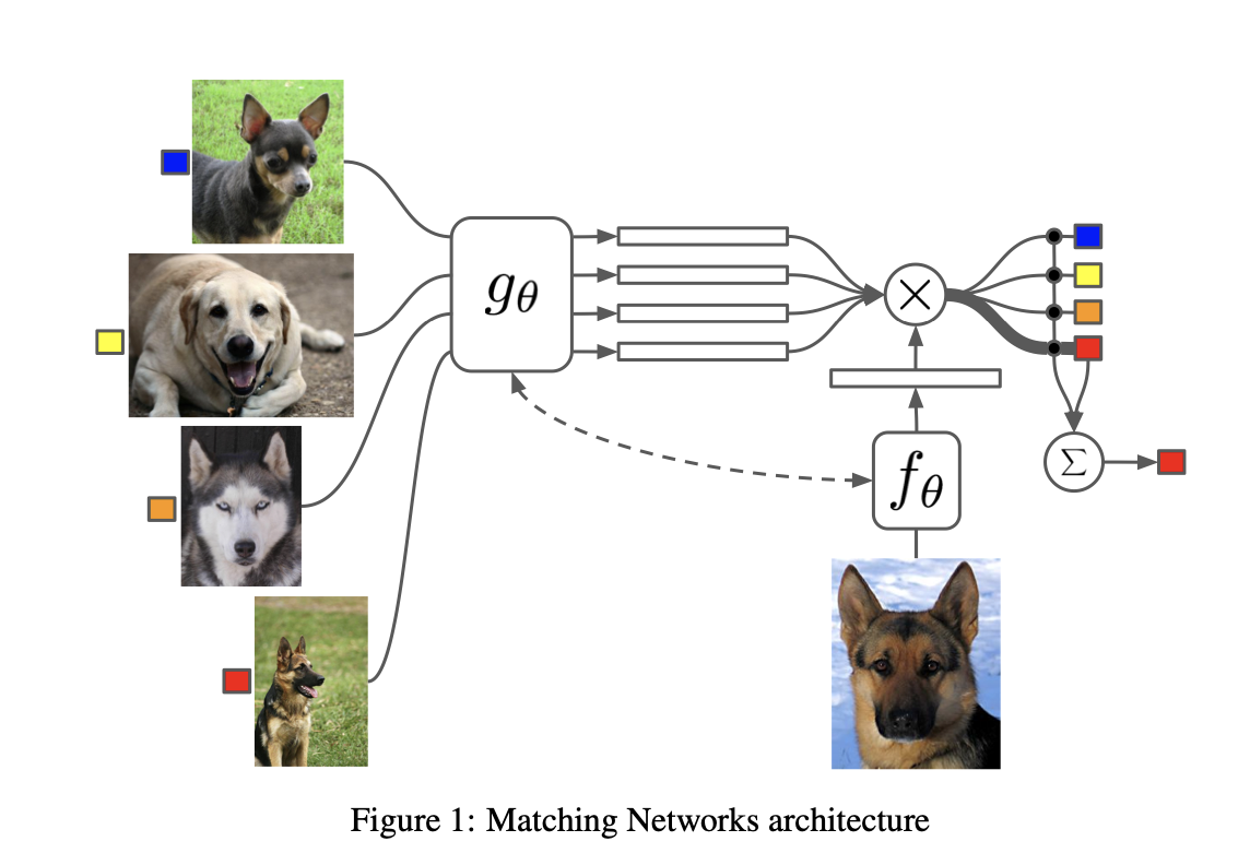
Training instances (here \(K=4\) different classes) are mapped into an embedding space. The mapping is realized by a neural network \(g\) with learnable parameters \(\Theta\). The query-image is also mapped to the same embedding space. The function \(f\) applied for mapping the query image need not be the same as the function \(g\). In the embedded space a simple nearest-neighbour search is applied to determine the class of the query image. I.e. for the given representation of the query-image the closest representation of a training image is determined. The class of this closest training image is the decision. The more similar tasks are available to learn the functions \(f\) and \(g\) the better the accuracy on similar tasks.
Cross Validation#
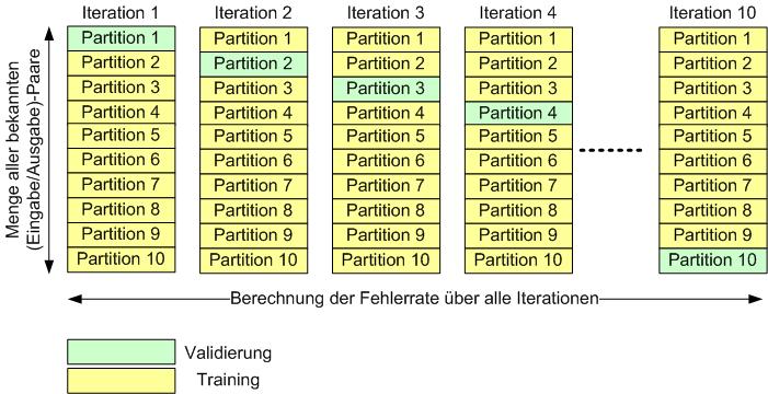
K-fold cross-Validation is the standard validation method if labeled data is rare. The entire set of labeled data is partitioned into k (\(k=10\) in the example below) disjoint subsets. The entire evaluation consists of k iterations. In the i.th iteration, the i.th partition (subset) is applied for validation, all other partitions are applied for training the model. In each iteration the model’s performance, e.g. accuracy, is determined on the validation-partition. Finally, the overall performance is the average performance over all k performance values.
Performance Metrics#
Below \(r_i\) denotes the true label, given in the labeled dataset and \(y_i\) denotes the corresponding label as predicted by the learned model. Obviously the goal is to learn a model, whose predictions \(y_i\) are as close as possible to the true labels \(r_i\). For classification and regression there exists different metrics to measure the difference between true and predicted labels. The most important metrics are summarized below. Metrics, provided by scikit-learn, can be found here: Scores in scikit-learn.
Classification#
For classification the most prominent metric is accuracy, which is just the rate of correct classifications. For the analysis of a classifier, determination of accuracy alone is not sufficient. The metrics defined below provide more subtle information on correct and erroneous events. All of the defined evaluation metrics can be obtained from the confusion matrix. For a binary classifier, the confusion matrix is depicted below. For a K-class classifier, the confusion matrix has size \(K \times K\). The rows correspond to the true labels, the columns to the predicted labels.

Accuracy: The rate of overall correct classifications:
Error Rate: The rate of overall erroneous classifications:
False Positive Rate:
True Positive Rate:
Precision: How much of the samples, which have been classified as positive are actual positive
Recall:(=TPR): How much of the true positive samples has been classified as positive
F1-Score: Harmonic mean of Precision and Recall
Regression#
Also regression models can be scored by a variety of metrics. The most prominent are
mean absolute error (MAE)
mean squared error (MSE)
median absolute error (MEDE)
coefficient of determination (\(R^2\))
If \(y_i\) is the predicted value for the i.th element and \(r_i\) is it’s true value, then these metrics are defined as follows:
Another frequently used regression metric is the Root Mean Squared Logarithmic Error (RMSLE), which is caluclated as follows:
For RMSLE there is no explicit scoring function in scikit-learn, but it can be easily computed via the NMSE-function. The RMSLE is well suited for the case that the error (i.e. the difference between \(y_i\) and \(r_i\)) increases with the values of \(r_i\). Then large errors at high values of \(r_i\) are weighted less by RMSLE.
Bias and Variance, Overfitting and Underfitting#
Bias-Variance-Tradeoff#
The goal of supervised machine learning is to learn a model
which maps inputs from \(\cal{X}\) to targets from \(\cal{Y}\) from a set of given training data \(T=\{x_p,y_p\}_{p=1}^N\) with \(x_p \in \cal{X}\) and \(y_p \in \cal{Y}\). The learned model \(f\), shall represent the deterministic part of the mapping from input \(x\) to target \(y\). However, in Machine Learning, it is assumed that this mapping contains also a non-deterministic prediction error \(\epsilon\), i.e.
The prediction error consists of the following 3 parts:
irreducible error
bias error
variance error
The irreducible error can not be avoided. It is caused, e.g. by latent variables, which influence the mapping but are not part of the input \(x\) or by erroneous measurements. However, bias-error and variance-error can be minimized by a careful selection and configuration of the ML algorithm. The ML engineer tries to learn a model, which minimizes both, bias- and variance-error.
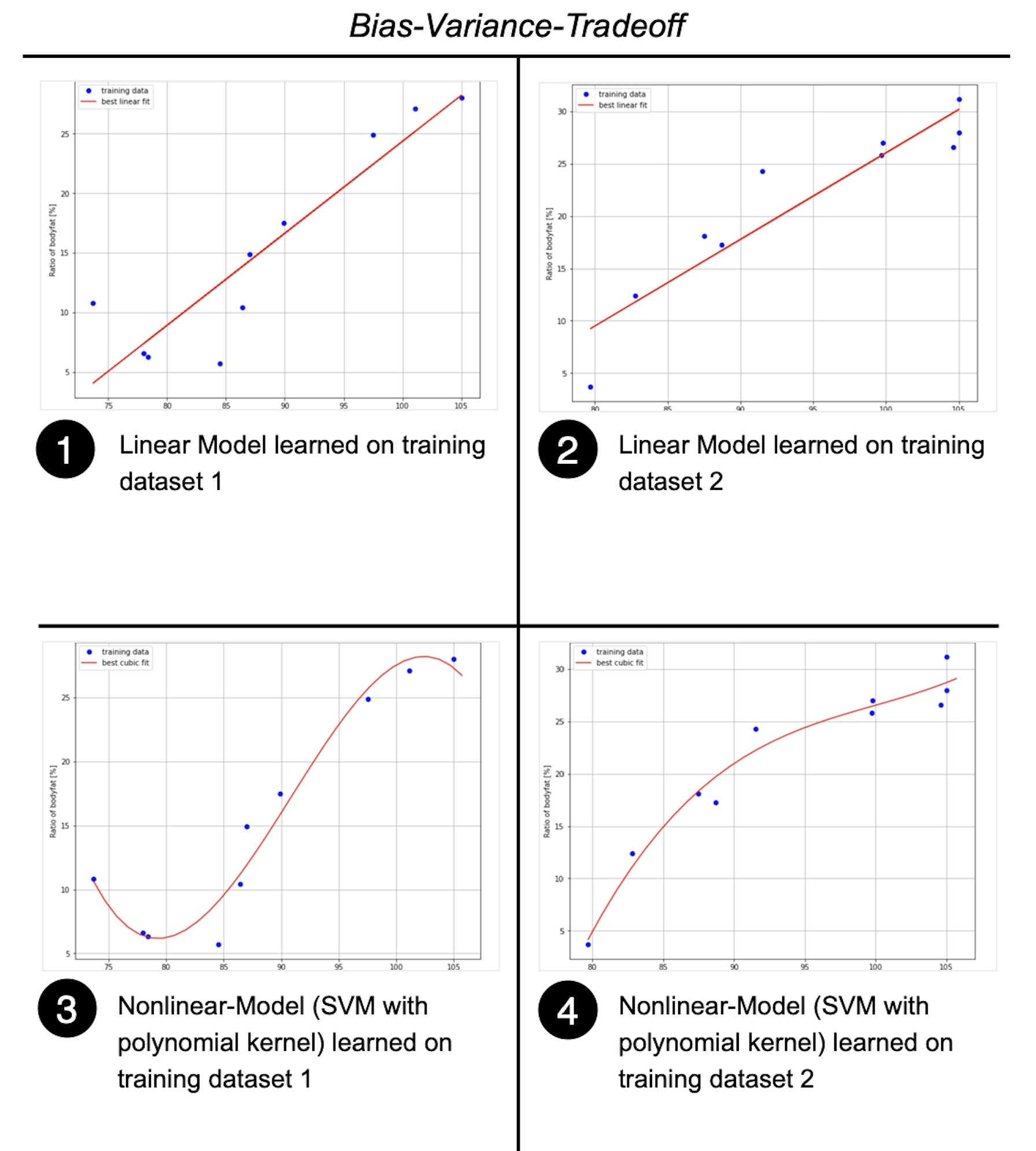
A high bias means that a learning algorithm has been selected, which imposes strict conditions on the type of the model, that can be learned. For example Linear Regression has a high bias, because only linear models can be learned. If the data can not be well fitted by such a linear model, the bias-error is high.
A high variance means that the learned model strongly varies with varying training data - even if the overall data distribution is identical. Algorithms, which are able to strongly adapt to the given training data are e.g. Support Vector Machines (SVM) with non-linear kernels or decision trees.
In the figure below the top-row (part 1 and part 2) shows a linear model of high bias (only a linear function can be learned). The variance is low because even though the training data in part 1 and part 2 is different, the learned models are similar. The lower row (part 3 and part 4) refers to an algorithm (non-linear SVM) of low-bias (many different types of functions can be learned), but high-variance, because the learned model in part 3 and part 4 are significantly different.
The goal is to find an algorithm, which learns a model of low bias and low variance. However, usually low bias yields high variance and vice versa. The goal is to find a good trade-off between them
Overfitting / Underfitting#
The goal of supervised machine learning is to find a model, which performs well on new data, i.e. data, which has not be seen during training. It is in general no problem, to find an algorithm, which learns a model, that is well adapted to the given training data. However, it is a big challenge to find a model, that performs well on previously unseen data.
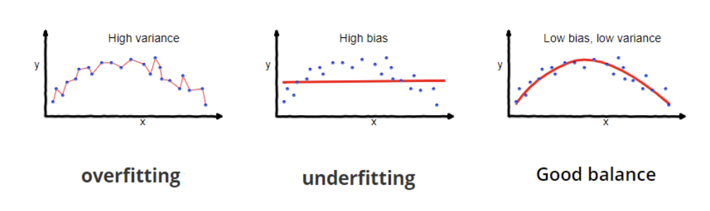
Overfitting means, that a model has been strongly adapted to the training data, but it performs bad on new data. Algorithms of low-bias are able to learn models, which are strongly fittet to training data. However, then often the variance and the probability of overfitting are high.
Underfitting means, that the learned model is weakly adapted to the training data. Algorithms of high-bias yield an increased probability of underfitting.
The image below sketches the relation between bias, variance, over- and underfitting (Image source: https://towardsdatascience.com/understanding-the-bias-variance-tradeoff-165e6942b229)
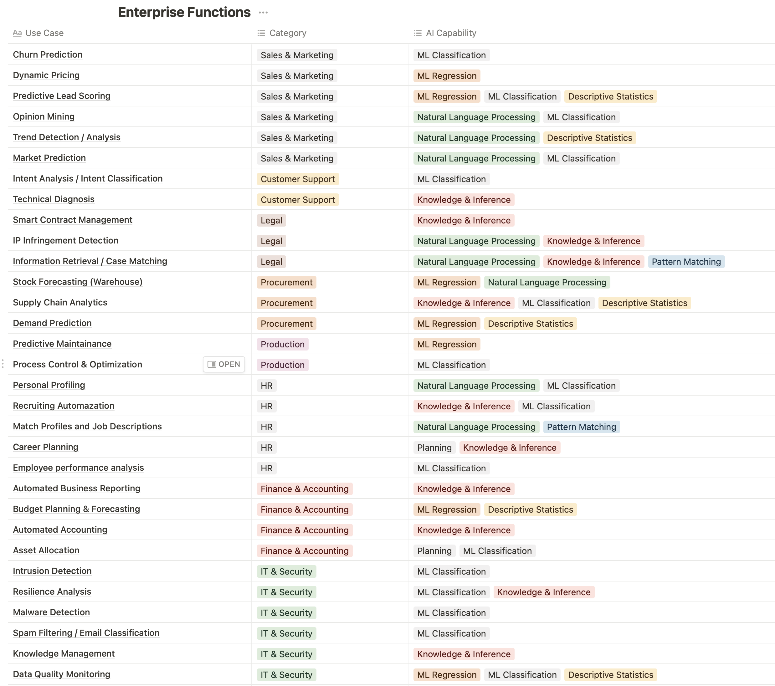
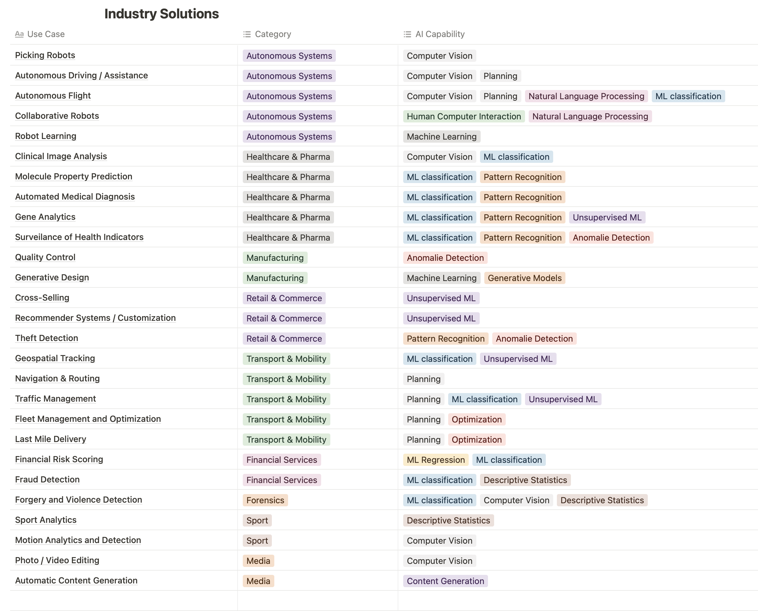
A incomplete list of AI Applications#
Current Problems/Challenges of AI and ML#
Data efficiency: In order to learn complex tasks large amounts of training data are required
Explainability/Interpretability: Models generate/predict an output for a given input, but they don’t explain why
Confidence: Many applications require that the model outputs not only a prediction but also confidence-measure.
Integrate Domain Knowledge: Neural Networks currently learn from data, but they are not able to integrate domain knowledge from experts. Integration of data- and expert-knowledge is desired.
Common Sense makes human learning efficient. It is hard to learn common sense knowledge in ML.
ML models usually learn correlations but not Causality.