Representations for Words and Texts

• Author: Johannes Maucher

• Last Update: 16.12.2020

In previous sections different types of data, numeric and categorial, have been applied. It has been shown how categorical data is mapped to numeric values or numeric vectors, such that it can be applied as input of a Machine Learning algorithm.

Another type of data is text, either single words, sentences, sections or entire documents. How to map these types to numeric representations?

One-Hot-Encoding of Single Words

A very simple option for representing single words as numeric vectors is One-Hot-Encoding. This type of encoding has already been introduced above for modelling non-binary categorial features. Each possible value (word) is uniquely mapped to an index, and the associated vector contains only zeros, except at the position of the value’s (word’s) index.

For example, assume that the entire set of possible words is

\[ V=(\mbox{all, and, at, boys, girls, home, kids, not, stay}). \]

Then a possible One-Hot-Encoding of these words is then

all	1	0	0	0	0	0	0	0	0
and	0	1	0	0	0	0	0	0	0
at	0	0	1	0	0	0	0	0	0
boys	0	0	0	1	0	0	0	0	0
girls	0	0	0	0	1	0	0	0	0
home	0	0	0	0	0	1	0	0	0
kids	0	0	0	0	0	0	1	0	0
not	0	0	0	0	0	0	0	1	0
stay	0	0	0	0	0	0	0	0	1

import pandas as pd

A word-index is just a one-to-one mapping of words to integers. Usually the word-index defines the One-Hot-Encoding of words: If \(i(w)\) is the index of word \(w\), then the One-Hot-Encoding of \(v(w)\) is a vector, which consists of only zeros, except at the element at position \(i(w)\). The value at this position is 1.

simpleWordDF=pd.DataFrame(data=["all", "and", "at", "boys", "girls", "home", "kids", "not", "stay"])
print("\nWord Index:")
simpleWordDF

Word Index:

	0
0	all
1	and
2	at
3	boys
4	girls
5	home
6	kids
7	not
8	stay

print("\nCorresponding One-Hot-Encoding")
pd.get_dummies(simpleWordDF,prefix="")

Corresponding One-Hot-Encoding

	_all	_and	_at	_boys	_girls	_home	_kids	_not	_stay
0	1	0	0	0	0	0	0	0	0
1	0	1	0	0	0	0	0	0	0
2	0	0	1	0	0	0	0	0	0
3	0	0	0	1	0	0	0	0	0
4	0	0	0	0	1	0	0	0	0
5	0	0	0	0	0	1	0	0	0
6	0	0	0	0	0	0	1	0	0
7	0	0	0	0	0	0	0	1	0
8	0	0	0	0	0	0	0	0	1

Word Embeddings

One-Hot-Encoding of words suffer from the following drawbacks:

1. The vectors are usually very long - there length is given by the number of words in the vocabulary.

2. The vectors are extremely sparse: only one non-zero entry.

3. Semantic relations between words are not modelled. This means that in this model there is no information about the fact that word car is more related to word vehicle than to word lake.

All of these drawbacks can be solved by applying Word Embeddings and by the way the resulting Word Embeddings are passed to neural networks.

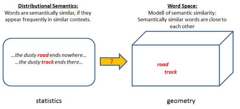
Word embeddings have revolutionalized many fields of Natural Language Processing since their efficient neural-network-based generation has been published in Efficient Estimation of Word Representations in Vector Space by Mikolov et al (2013). Word embeddings map words into vector-spaces such that semantically or syntactically related words are close together, whereas unrelated words are far from each other. Moreover, it has been shown that the word-embeddings, generated by word2vec-techniques CBOW or Skipgram, are well-structured in the sense that also relations such as is-capital-of, is-female-of, is-plural-of are encoded in the vector space. In this way questions like woman is to queen, as man is to ? can be answered by simple operations of linear algebra in the word-vector-space. Compared to the length of one-hot encoded word-vectors, word-embedding-vectors are short (typical lengths in the range from 100-300) and dense (float-values).

CBOW and Skipgram, are techniques to learn word-embeddings, i.e. a mapping of words to vectors by relatively simple neural networks. Usually large corpora are applied for learning, e.g. the entire Wikipedia corpus in a given language. Today, pretrained models for the most common languages are available, for example from FastText project.

Bag of Word Modell of documents

Term Frequencies

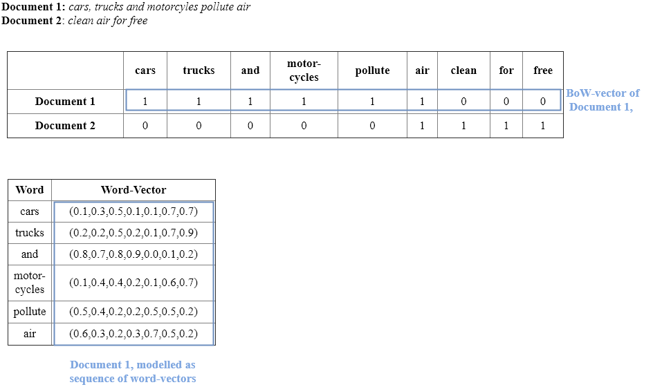
The conventional model for representing texts of arbitrary length as numeric vectors, is the Bag-of-Words model. In this model each word of the underlying vocabulary corresponds to one column and each document (text) corresponds to a single row of a matrix. The entry in row \(i\), column \(j\) is just the term-frequency \(tf_{i,j}\) of word \(j\) in document \(i\).

For example, assume, that we have only two documents

• Document 1: not all kids stay at home

• Document 2: all boys and girls stay not at home

The BoW model of these documents is then

	all	and	at	boys	girls	home	kids	not	stay
Document 1	1	0	1	0	0	1	1	1	1
Document 2	1	1	1	1	1	1	0	1	1

from sklearn.feature_extraction.text import CountVectorizer
vectorizer = CountVectorizer()

corpus = ['not all kids stay at home.',
          'all boys and girls stay not at home.',
         ]
BoW = vectorizer.fit_transform(corpus)
vectorizer.get_feature_names()

['all', 'and', 'at', 'boys', 'girls', 'home', 'kids', 'not', 'stay']

BoW.toarray()

array([[1, 0, 1, 0, 0, 1, 1, 1, 1],
       [1, 1, 1, 1, 1, 1, 0, 1, 1]])

Term Frequency Inverse Document Frequency

Instead of the term-frequency \(tf_{i,j}\) it is also possible to fill the BoW-vector with

• a binary indicator which indicates if the term \(j\) appears in document \(i\)

• the tf-idf-values

\[ tfidf_{i,j}=tf_{i,j} \cdot log \frac{N}{df_j}, \]

where \(df_j\) is the frequency of documents, in which term \(j\) appears, and \(N\) is the total number of documents. The advantage of tf-idf, compared to just tf-entries, is that in tf-idf the term-frequency tf is multiplied by a value idf, which is small for less informative words, i.e. words which appear in many documents, and high for words, which appear in only few documents. It is assumed, that words, which appear only in a few documents have a stronger semantic focus and are therefore more important.

from sklearn.feature_extraction.text import TfidfVectorizer
vectorizer = TfidfVectorizer()

tfidf_BoW = vectorizer.fit_transform(corpus)

tfidf_BoW.toarray()

array([[0.37863221, 0.        , 0.37863221, 0.        , 0.        ,
        0.37863221, 0.53215436, 0.37863221, 0.37863221],
       [0.30253071, 0.42519636, 0.30253071, 0.42519636, 0.42519636,
        0.30253071, 0.        , 0.30253071, 0.30253071]])

As can be seen in the example above, words which appear in all documents are weighted by 0, i.e. they are considered to be not relevant.

How to generate Wordembeddings? CBOW and Skipgram

In 2013 Mikolov et al. published Efficient Estimation of Word Representations in Vector Space. They proposed quite simple neural network architectures to efficiently create word-embeddings: CBOW and Skipgram. These architectures are better known as Word2Vec. In both techniques neural networks are trained for a pseudo-task. After training, the network itself is usually not of interest. However, the learned weights in the input-layer constitute the word-embeddings, which can then be applied for a large field of NLP-tasks, e.g. document classification.

Continous Bag-Of-Words (CBOW)

The idea of CBOW is to predict the target word \(w_i\), given the \(N\) context-words \(w_{i-N/2},\ldots, w_{i-1}, \quad w_{i+1}, w_{i+N/2}\). In order to learn such a predictor a large but unlabeled corpus is required. The extraction of training-samples from a corpus is sketched in the picture below:

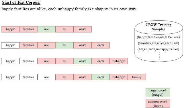
In this example a context length of \(N=4\) has been applied. The first training-element consists of

• the \(N=4\) input-words (happy,families,all,alike)

• the target word are.

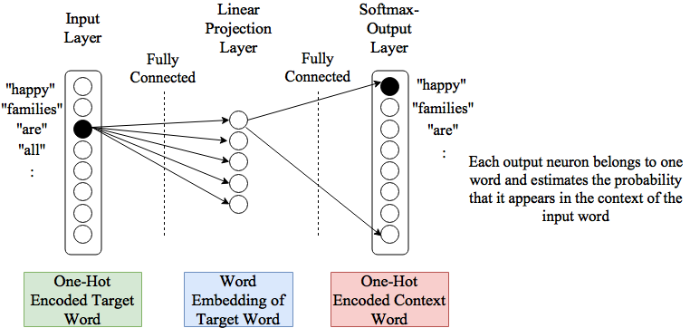
In order to obtain the second training-sample the window of length \(N+1\) is just shifted by one to the right. The concrete architecture for CBOW is shown in the picture below. At the input the \(N\) context words are one-hot-encoded. The fully-connected Projection-layer maps the context words to a vector representation of the context. This vector representation is the input of a softmax-output-layer. The output-layer has as much neurons as there are words in the vocabulary \(V\). Each neurons uniquely corresponds to a word of the vocabulary and outputs an estimation of the probaility, that the word appears as target for the current context-words at the input.

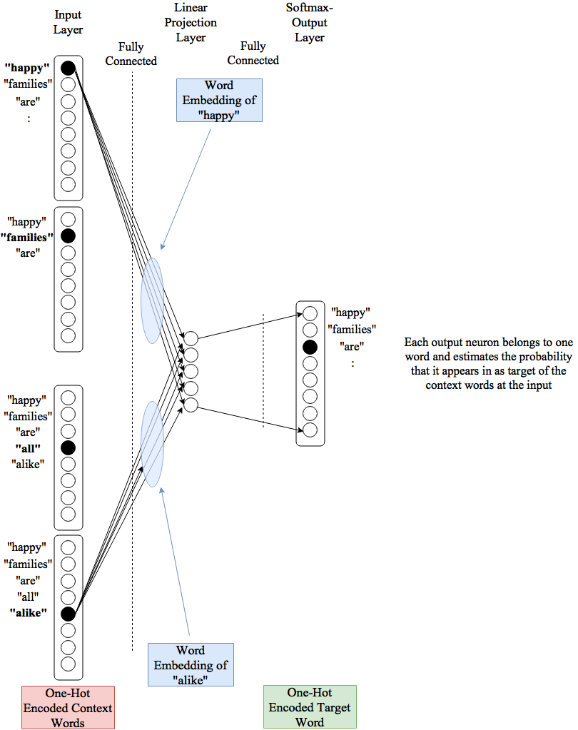
After training the CBOW-network the vector representation of word \(w\) are the weights from the one-hot encoded word \(w\) at the input of the network to the neurons in the projection-layer. I.e. the number of neurons in the projection layer define the length of the word-embedding.

Skip-Gram

Skip-Gram is similar to CBOW, but has a reversed prediction process: For a given target word at the input, the Skip-Gram model predicts words, which are likely in the context of this target word. Again, the context is defined by the \(N\) neighbouring words. The extraction of training-samples from a corpus is sketched in the picture below:

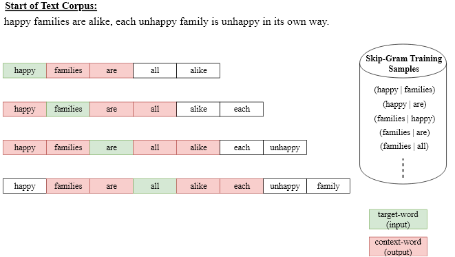
Again a context length of \(N=4\) has been applied. The first training-element consists of

• the first target word (happy) as input to the network

• the first context word (families) as network-output.

The concrete architecture for Skip-gram is shown in the picture below. At the input the target-word is one-hot-encoded. The fully-connected Projection-layer outputs the current vector representation of the target-word. This vector representation is the input of a softmax-output-layer. The output-layer has as much neurons as there are words in the vocabulary \(V\). Each neurons uniquely corresponds to a word of the vocabulary and outputs an estimation of the probaility, that the word appears in the context of the current target-word at the input.

Other Word-Embeddings

CBOW- and Skip-Gram are possibly the most popular word-embeddings. However, there are more count-based and prediction-based methods to generate them, e.g. Random-Indexing, Glove, FastText.

How to Access Pretrained Word-Embeddings?

Fasttext Word-Embeddings

After downloading word embeddings from FastText they can be imported as follows:

from gensim.models import KeyedVectors

# Creating the model
#en_model = KeyedVectors.load_word2vec_format('/Users/maucher/DataSets/Gensim/FastText/Gensim/FastText/wiki-news-300d-1M.vec')
#en_model = KeyedVectors.load_word2vec_format(r'C:\Users\maucher\DataSets\Gensim\Data\Fasttext\wiki-news-300d-1M.vec\wiki-news-300d-1M.vec') #path on surface
en_model = KeyedVectors.load_word2vec_format('/Users/johannes/DataSets/Gensim/FastText/fasttextEnglish300.vec')
# Getting the tokens 
words = []
for word in en_model.key_to_index:
    words.append(word)

# Printing out number of tokens available
print("Number of Tokens: {}".format(len(words)))

# Printing out the dimension of a word vector 
print("Dimension of a word vector: {}".format(
    len(en_model[words[0]])
))

Number of Tokens: 999994
Dimension of a word vector: 300

print(words[100])
print("First 10 components of word-vector: \n",en_model[words[100]][:10])

than
First 10 components of word-vector: 
 [ 0.1016 -0.1216 -0.0356  0.0096 -0.1015  0.1766 -0.0593  0.032   0.0892
 -0.0727]

The KeyedVectors-class provides many interesting methods on word-embeddings. For example the most_similar(w)-methode returns the words, whose word-vectors match best with the word-vector of w:

en_model.most_similar("car")

[('cars', 0.8045914769172668),
 ('automobile', 0.7667388916015625),
 ('vehicle', 0.7534858584403992),
 ('Car', 0.7177953124046326),
 ('truck', 0.6989946961402893),
 ('SUV', 0.6896128058433533),
 ('automobiles', 0.6783526539802551),
 ('dealership', 0.6682883501052856),
 ('garage', 0.6681075096130371),
 ('driver', 0.6541329026222229)]

Glove Word-Embeddings

After downloading word-embeddings from Glove, they can be imported as follows:

import os
import numpy as np
#GLOVE_DIR = "./Data/glove.6B"
#GLOVE_DIR ="/Users/maucher/DataSets/glove.6B"
GLOVE_DIR = '/Users/johannes/DataSets/Gensim/glove/'

from gensim.test.utils import datapath, get_tmpfile
from gensim.models import KeyedVectors
from gensim.scripts.glove2word2vec import glove2word2vec

glove_file = datapath(os.path.join(GLOVE_DIR, 'glove.6B.100d.txt'))
tmp_file = get_tmpfile(os.path.join(GLOVE_DIR, 'test_word2vec.txt'))

_ = glove2word2vec(glove_file, tmp_file)
model = KeyedVectors.load_word2vec_format(tmp_file)

<ipython-input-32-b7985f974e25>:8: DeprecationWarning: Call to deprecated `glove2word2vec` (KeyedVectors.load_word2vec_format(.., binary=False, no_header=True) loads GLoVE text vectors.).
  _ = glove2word2vec(glove_file, tmp_file)

model.most_similar("car")

[('vehicle', 0.8630837798118591),
 ('truck', 0.8597878813743591),
 ('cars', 0.837166965007782),
 ('driver', 0.8185911178588867),
 ('driving', 0.781263530254364),
 ('motorcycle', 0.7553156614303589),
 ('vehicles', 0.7462257146835327),
 ('parked', 0.74594646692276),
 ('bus', 0.737270712852478),
 ('taxi', 0.7155269384384155)]

Comparision: BoW vs. Sequence of Word-Embeddings

BoW representations of text suffer from crucial drawbacks:

1. The vectors are usually very long - there length is given by the number of words in the vocabulary. Moreover, the vectors are quite sparse, since the set of words appearing in one document is usually only a very small part of the set of all words in the vocabulary.

2. Semantic relations between words are not modelled. This means that in this model there is no information about the fact that word car is more related to word vehicle than to word lake.

3. In the BoW-model of documents word order is totally ignored. E.g. the model can not distinguish if word not appeared immediately before word good or before word bad.

All of these drawbacks can be solved by

• applying Word Embeddings

• passing sequences of Word-Embedding-Vectors to the input of

  • Recurrent Neural Networks,

  • Convolutional Neural Networks

  • Transformers