
K - Nearest Neighbour Classification / Regression
Contents
K - Nearest Neighbour Classification / Regression#
Probably the simplest supervised Machine Learning algorithm is K-Nearest Neighbour (K-NN). K-NN can be applied for both, classification and regression. Compared to other ML algorithms, K-NN is special because it is a non-parameteric ML algorithm, which actually has no training phase. It is therefore also called a Lazy Learner. All other ML algorithms, which will be introduced in this lecture, have a learning-phase during which either a class-specific data-distribution or a class-boundary is learned. After this learning phase the entire knowledge from the training-data set is encoded in some parameters, which uniquely define the class-specific distribution or the class-boundary. Not so with K-NN! In K-NN the entire set of labeled training data is stored. In the inference phase new data is classified by just comparing the new instance with all training-instances and deciding for the class, which most often appears in the set of k nearest training instances.
K-NN Classifier:
Training: Store the set of labeled training data \(T=\lbrace \mathbf{x}_t,r_t) \rbrace_{t=1}^N\)
Inference:
For a new input vector \(\mathbf{x}\): Determine the set \(M(\mathbf{x},T,K)\) of \(K\) training instances from \(T\), which are closest to \(\mathbf{x}\).
Assign the class \(r\) to \(\mathbf{x}\), which most often appears in \(M(\mathbf{x},T,K)\).
The number of neighbours \(K\) is a hyperparameter. If \(K\) is small (e.g. 1 or 3), the classifier is not robust w.r.t. outliers and possibly overfitted to training data. The higher the value of \(K\), the smoother the class boundary and the better the generalisation. However, a too high value may yield underfitting.
Another important hyperparameter is the distance-function, e.g. Euclidean-, Manhattan- or any other Minkowski-distance.
K-NN Regression:
Training: Store the set of labeled training data \(T=\lbrace \mathbf{x}_t,r_t) \rbrace_{t=1}^N\)
Inference:
For a new input vector \(\mathbf{x}\): Determine the set \(M(\mathbf{x},T,K)\) of \(K\) training instances from \(T\), which are closest to \(\mathbf{x}\).
Assign the value \(r\) to \(\mathbf{x}\) by interpolating over the values in \(M(\mathbf{x},T,K)\).
For K-NN regression an additional hyperparameter is the interpolation method used to calculate the new value \(r\). The simplest method is to just take the arithmetic mean over the values in the neighborhood.
K-NN Pros and Cons:
The drawbacks of K-NN are
the large memory footprint, since all training data must be kept
long inference time, since each new instance must be compared to all training instances in order to determine the nearest neighbours
For \(K=1\) the bias is close to 0, but the variance is quite high. With increasing \(K\) bias increases but variance decreases.
K-NN Classification Demo#
In the reminder of this section the application of a K-NN classifier is demonstrated.
Generate set of labeled training data#
In this demo we do not apply a real-world training data set. Instead we generate Gaussian-distributed 2-dimensional training vectors \(\mathbf{x}=(x_1,x_2)\) for each of the 2 classes. The distributions of the 2 classes differ in their mean-vector and their covariance matrix. The code cells below implement the generation and visualisation of labeled data.
import numpy as np
from matplotlib import pyplot as plt
np.set_printoptions(precision=2)
from matplotlib.colors import ListedColormap
import seaborn as sns
Generate Gaussian-distributed 2-dimensional data for class 0:
np.random.seed(1234)
Numpoints=200
m1=1    #Mean of first dimension
m2=2    #Mean of second dimension
mean=np.array(([m1,m2]))
s11=1.7 #standard deviation of x1
s22=1.4 #standard deviation of x2
rho=0.8 #correlation coefficient between s11 and s22
#Determine covariance matrix from standard deviations
var11=s11**2
var22=s22**2
var12=rho*s11*s22
var21=var12
cov=np.array(([var11,var12],[var21,var22]))
print("Configured mean: ")
print(mean)
print("Configured covariance: ")
print(cov)
pointset0=np.random.multivariate_normal(mean,cov,Numpoints,)
print("First samples of pointset:")
print(pointset0[:20,:])
Configured mean:
[1 2]
Configured covariance:
[[2.89 1.9 ]
 [1.9  1.96]]
First samples of pointset:
[[ 0.73  0.75]
 [-1.23 -0.02]
 [ 1.81  3.41]
 [-0.15  0.55]
 [ 1.92  0.78]
 [-1.31  1.04]
 [ 0.28 -0.32]
 [ 1.55  2.43]
 [ 0.21  1.63]
 [-0.52 -0.54]
 [ 1.61  1.91]
 [ 0.45  2.05]
 [-0.97  0.04]
 [ 0.65  0.15]
 [ 0.86  2.8 ]
 [ 1.51  2.7 ]
 [-1.17  1.21]
 [-0.37  0.82]
 [ 0.93  1.67]
 [-1.39  2.19]]
Generate Gaussian-distributed 2-dimensional data for class 1:
Numpoints=200
m1=-2    #Mean of first dimension
m2=3   #Mean of second dimension
mean=np.array(([m1,m2]))
s11=0.8 #standard deviation of x1
s22=0.4 #standard deviation of x2
rho=0.1 #correlation coefficient between s11 and s22
#Determine covariance matrix from standard deviations
var11=s11**2
var22=s22**2
var12=rho*s11*s22
var21=var12
cov=np.array(([var11,var12],[var21,var22]))
print("Configured mean: ")
print(mean)
print("Configured covariance: ")
print(cov)
pointset1=np.random.multivariate_normal(mean,cov,Numpoints)
print("First samples of pointset:")
print(pointset1[:20,:])
Configured mean:
[-2  3]
Configured covariance:
[[0.64 0.03]
 [0.03 0.16]]
First samples of pointset:
[[-1.79  2.65]
 [-2.25  2.48]
 [-1.83  2.83]
 [-2.83  3.5 ]
 [-2.88  3.12]
 [-1.26  3.54]
 [-2.39  2.72]
 [-1.43  2.94]
 [-2.48  3.11]
 [-0.52  2.74]
 [-1.4   3.  ]
 [-2.23  3.08]
 [-1.78  2.89]
 [-2.36  2.95]
 [-1.63  3.16]
 [-1.17  2.93]
 [-3.09  2.43]
 [-0.79  3.7 ]
 [-1.52  2.96]
 [-3.32  2.7 ]]
Assign class labels and vertically stack class 0 and class 1 data. The array of all input vectors is \(X\) and the vector of all labels is \(y\). The class-index of the \(i.th\) row in \(X\) is the value of the \(i.th\) component in \(y\):
X=np.vstack([pointset0,pointset1])
y=np.transpose(np.hstack([np.zeros(Numpoints),np.ones(Numpoints)]))
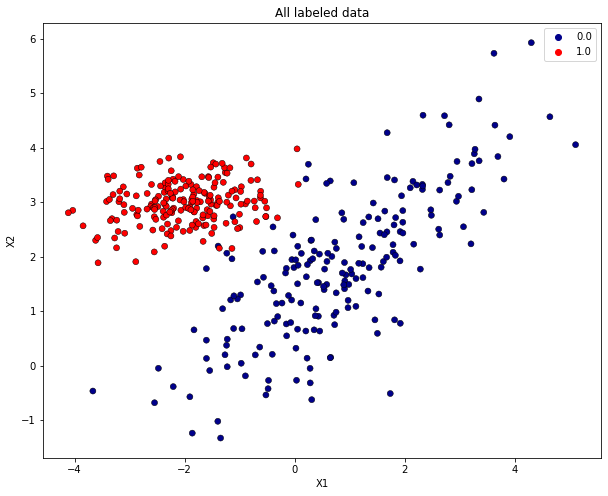
Visualize all labeled data. Data of class 0 has blue, data of class 1 red markers.
h = .02  # step size in the mesh
# Create color maps
cmap_light = ListedColormap(['cornflowerblue','orange'])
cmap_bold = ['darkblue','red']
plt.figure(figsize=(10, 8))
sns.scatterplot(x=X[:, 0], y=X[:, 1],hue=y,palette=cmap_bold, alpha=1.0, edgecolor="black")
plt.title("All labeled data")
plt.xlabel("X1")
plt.ylabel("X2")
plt.show()
Split labeled data in training- and test-partition#
The scikit-learn function train_test_split() shuffles the set of all labeled data and returns two partions of input vectors, X_train and X_test and the corresponding class-labels y_train and y_test.
from sklearn.model_selection import train_test_split
from sklearn import neighbors
X.shape
(400, 2)
y.shape
(400,)
X_train, X_test, y_train, y_test = train_test_split(X, y, test_size=0.3, random_state=412)
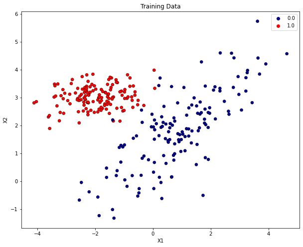
Visualize training data: The plot below contains only those input-vectors from \(X\), which has been assigned to the training-partition \(X\).
plt.figure(figsize=(10, 8))
sns.scatterplot(x=X_train[:, 0], y=X_train[:, 1],hue=y_train,palette=cmap_bold, alpha=1.0, edgecolor="black")
plt.title("Training Data")
plt.xlabel("X1")
plt.ylabel("X2")
plt.show()
Train the K-NN classifier#
All machine learning algorithms implemented in scikit-learn provide a .fit(X_train, y_train)-method, in which the training phase, i.e. the fitting of a model to the given training-data, is implemented. As already described above, in the case of the K-NN algorithm, there is no training-phase. Here, fit() just saves the given training data accordingly. The model is the set of training data itself. In this example the chosen number of neighbors is \(K=3\).
K=3
clf = neighbors.KNeighborsClassifier(K)
clf.fit(X_train, y_train)
KNeighborsClassifier(n_neighbors=3)
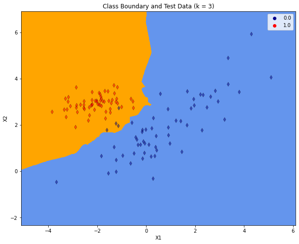
After training the resulting class boundary is plotted. The plot also contains the test-data. For plotting the decision boundary a class-specific color will be assigned to each point in the mesh \([x_{min}, x_{max}] \times [y_{min}, y_{max}]\).
x_min, x_max = X[:, 0].min() - 1, X[:, 0].max() + 1
y_min, y_max = X[:, 1].min() - 1, X[:, 1].max() + 1
xx, yy = np.meshgrid(np.arange(x_min, x_max, h),
                     np.arange(y_min, y_max, h))
Z = clf.predict(np.c_[xx.ravel(), yy.ravel()])

# Put the result into a color plot
Z = Z.reshape(xx.shape)
plt.figure(figsize=(10, 8))
plt.contourf(xx, yy, Z, cmap=cmap_light)

# Plot also the test points
sns.scatterplot(x=X_test[:, 0], y=X_test[:, 1],hue=y_test,palette=cmap_bold,marker="d",alpha=0.5,edgecolor="black")
plt.xlim(xx.min(), xx.max())
plt.ylim(yy.min(), yy.max())
plt.title("Class Boundary and Test Data (k = %i)"% (K))
plt.xlabel("X1")
plt.ylabel("X2")
plt.show()
Evaluate the classifier on Test-data#
y_pred=clf.predict(X_test)
from sklearn.metrics import accuracy_score,confusion_matrix
accuracy_score(y_test,y_pred)
0.9666666666666667
confusion_matrix(y_test,y_pred)
array([[56,  4],
       [ 0, 60]])
As can be seen in the confusion matrix, all class-1 data has been classified correctly. But there are 4 out of 60 class-0 instances, which are assigned to the wrong class. In the visualisation above, these errors are the blue markers in the orange region.
Repeat Training and Evaluation for \(K=9\) neighbors#
K=7
clf = neighbors.KNeighborsClassifier(K)
clf.fit(X_train, y_train)
KNeighborsClassifier(n_neighbors=7)
x_min, x_max = X[:, 0].min() - 1, X[:, 0].max() + 1
y_min, y_max = X[:, 1].min() - 1, X[:, 1].max() + 1
xx, yy = np.meshgrid(np.arange(x_min, x_max, h),
np.arange(y_min, y_max, h))
Z = clf.predict(np.c_[xx.ravel(), yy.ravel()])
# Put the result into a color plot
Z = Z.reshape(xx.shape)
plt.figure(figsize=(10, 8))
plt.contourf(xx, yy, Z, cmap=cmap_light)
# Plot also the test points
sns.scatterplot(x=X_test[:, 0], y=X_test[:, 1],hue=y_test,palette=cmap_bold,marker="d",alpha=0.5,edgecolor="black")
plt.xlim(xx.min(), xx.max())
plt.ylim(yy.min(), yy.max())
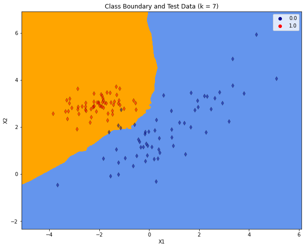
plt.title("Class Boundary and Test Data (k = %i)"% (K))
plt.xlabel("X1")
plt.ylabel("X2")
plt.show()
y_pred=clf.predict(X_test)
accuracy_score(y_test,y_pred)
0.9666666666666667
confusion_matrix(y_test,y_pred)
array([[56,  4],
       [ 0, 60]])
As the plot above shows, for the increased \(K\) the class-boundary becomes smoother. But there are still 4 misclassified instances in the test-partition.