Generative Adversarial Nets (GAN)

In 2014 GANs have been introduced by Ian Goodfellow in [GPAM+14] (Ian Goodfellow et al). Since then they are one of the hottest topics in deeplearning research. GANs are able to generate synthetic data that looks similar to data of a given trainingset. In this way artifical images, paintings, texts, audio or handwritten digits can be generated.

Idea GANs

On an abstract level the idea of GANs can be described as follows: A counterfeiter produces fake banknotes. The police is able to discriminate the fake banknotes from real ones and it provides feedback to the counterfeiter on why the banknotes can be detected as fake. This feedback is used by the counterfeiter in order to produce fake, which is less distinguishable from real bankotes. After some iterations of producing better but not sufficiently good fake the counterfeiter is able to produce fake, which can not be discriminated from real banknotes.

A GAN consists of two models:

1. The discriminator is the police. It learns to discriminate real data from artificially generated fake data.

2. The generator is the counterfeiter, which learns to generate data, that is indistinguishable from real data.

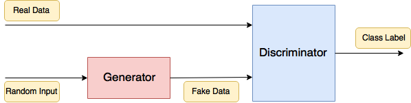
Fig. 31 GAN: Generator-Network tries to produce data, such that the Discriminator-Network can not distinguish this fake-data from real-data.

Architecture and Training

As depicted in image GAN overall picture the overall GAN consists of a Generator and a Discriminator. Both of them are usually neural networks of any type. In the initial work [GPAM+14] MLPs have been applied for both components. Later, it has been shown in [RMC16], that GANs, which apply CNNs for both components are much easier to configure and behave in a more stable manner. The CNN, which has been applied as Generator in [RMC16], is depicted below:

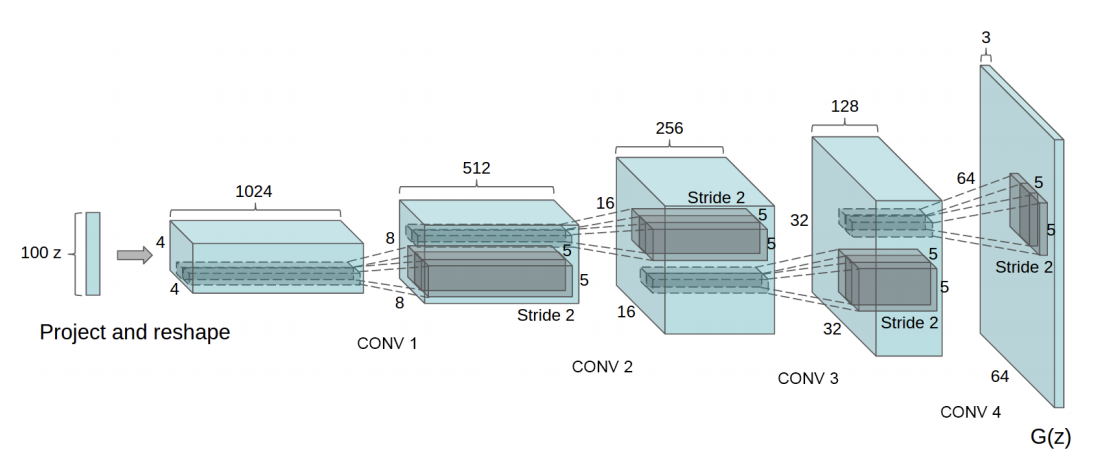
Fig. 32 Generator of the DCGAN. Image Source: [RMC16]. The upsizing of the feature maps is realized by fractional-strided convolution. This is what has be denoted by Deconvolution with a stride \(>2\) in notebook Animations of Convolution and Deconvolution

The task of the GAN is to generate fake-data at the output of the Generator. This fake data shall be indistinguishable from the real-data \(\mathbf{x}\), which is passed to the Discriminator input. The input to the Generator is usually a random noise vector \(\mathbf{z}\), drawn e.g. from a multivariate Gaussian distribution. The Generator must be designed such that it’s output \(G(\mathbf{z})\) has the same format as the real-data at the input of the discriminator. The Discriminator is a binary classification network, which receives real-data \(\mathbf{x}\) and fake-data \(G(\mathbf{z})\), provided by the Generator. The Discriminator is trained such, that it can discriminate fake-data from real-data. The Generator is trained such, that its output \(G(\mathbf{z})\) is not distinguishable from real-data, i.e. both networks have adversarial training goals.

The adversarial training process is depcited in the flow-chart below. In each epoch

1. First the discriminator is trained with a batch of real- and fake-data. For this

   • real-data \(x\) is labeled by \(1\)

   • fake-data \(G(z)\) is labeled by \(0\)

   In this phase the weight in the discriminator are adapted such that the Minmax-Loss

   (71)\[ E_x \left[ \log(D(x)) \right] + E_z \left[ log(1-D(G(z))) \right] \]

   is maximized. In this equation

   • \(D(x)\) is the Discriminator’s estimate of the probability that real data instance \(x\) is real.

   • \(E_x\) is the Expected value over all real data instances.

   • \(G(z)\) is the Generator’s output when given noise \(z\).

   • \(D(G(z))\) is the Discriminator’s estimate of the probability that a fake instance is real.

   • \(E_z\) is the Expected value over all random inputs to the generator.

   For a minibatch of \(m\) real-data samples \(\lbrace x^{(1)}, \ldots, x^{(m)} \rbrace\) and \(m\) random samples \(\lbrace z^{(1)}, \ldots, z^{(m)} \rbrace\), the expected values in equation (71)are calculated by

   (72)\[ \frac{1}{m} \sum\limits_{i=1}^m \left[ \log(D(x^{(i)})) + log(1-D(G(z^{(i)}))) \right] \]

2. The weights of the Discrimator are being frozen and the Generator is trained. For this a minibatch of \(m\) random-noise vectors \(\lbrace z^{(1)}, \ldots, z^{(m)} \rbrace\) is sampled and passed to the generator. The Generator outputs \(G(z^{(i)})\) are now labeled by 1 and passed to the Discriminator. In this phase only the weights of the Generator are adapted. They are adapted such that the Minmax-loss of equation (71) is minimized. For a minibatch of \(m\) random samples \(\lbrace z^{(1)}, \ldots, z^{(m)} \rbrace\), the following Loss is minimized during Generator training:

   (73)\[ \frac{1}{m} \sum\limits_{i=1}^m log(1-D(G(z^{(i)}))). \]

Fig. 33 GAN training process.

Even if CNNs are applied as Generator and Discriminator, the configuration of GANs remains challenging. The authors of [RMC16] recommend the guidelines given below:

Fig. 34 Source: [RMC16]

Conditional GAN

In [MO14] conditional GANs (cGAN) has been introduced. cGANs allow to control different variants of the generated fake-data. For example, if MNIST-like handwritten digits shall be generated by the GAN one can control which concrete digit shall be generated. The control is realized by passing additional information \(y\) to both, the input of the Generator and the input of the Discriminator.

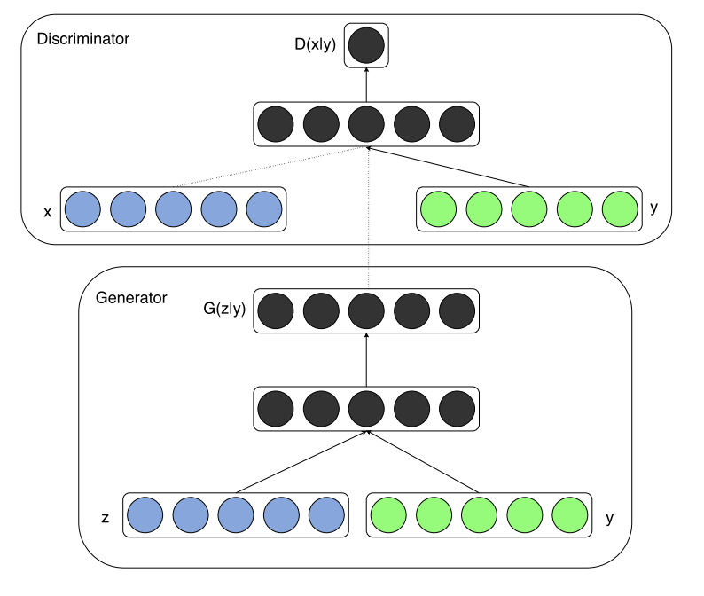
Fig. 35 Conditional GAN: The condition \(y\) is added to the Generator- and Discriminator input. Depending on the condition different fake-data \(G(z)\) can be generated. Source: [MO14]

For conditional GANs the Minmax-Loss Function, which is maximized by the Discriminator- and minimized by the Generator-training is

(74)\[ E_x \left[ \log(D(x \mid y)) \right] + E_z \left[ \log(1-D(G(z \mid y))) \right] \]

In the MNIST-example \(y\) represents the concrete number, e.g. it is the one-hot-encoding of the digit that shall be generated. In general, \(y\) can be any kind of auxillary information, such as a class-label or data from other modalities, e.g. word-vectors.

Fig. 36 Source: [MO14]

Cycle GAN: Transform from one domain to another

Image-to-image translation (see picture below for examples) is a class of vision- and graphics-problems, where the goal is to learn the mapping between an input image and an output image using a training set of aligned image pairs. However, for many tasks, paired training data may not be available [ZPIE17].

Fig. 37 Source: [ZPIE17].

Cycle GAN, as introduced in [ZPIE17], is an approach for learning to translate an image from a source domain \(X\) to a target domain \(Y\) without requiring paired images for training - two sets of unpaired images are sufficient.

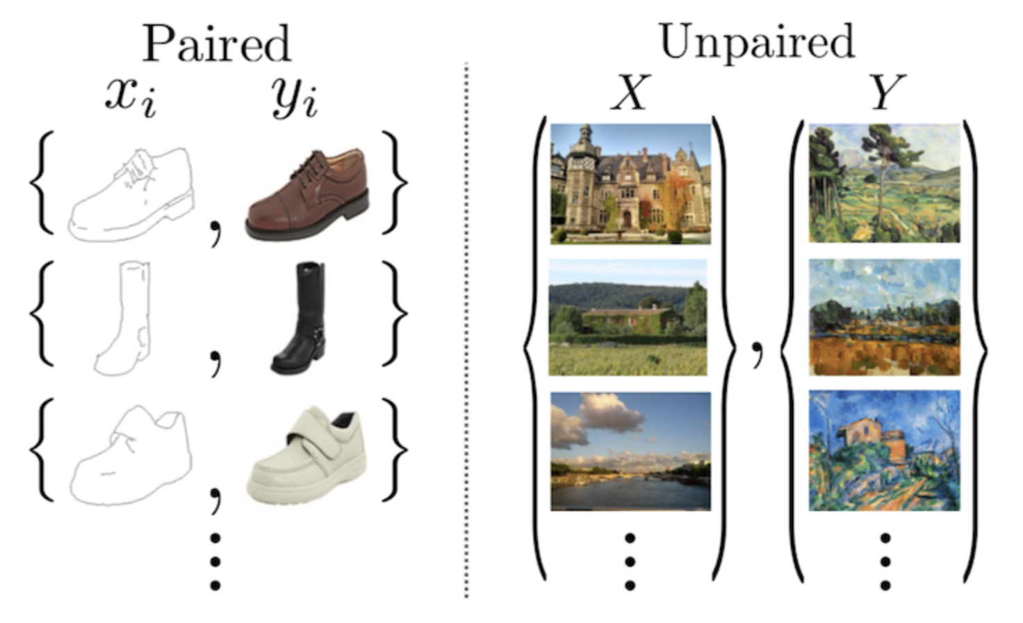
Fig. 38 Paired vs. unpaired training data. For Cycle GAN unpaired data is sufficient. Source: [ZPIE17].

In Cycle GAN a mapping

\[ G : X \rightarrow Y \]

is learned, such that the distribution of images from \(G(X)\) is indistinguishable from the distribution \(Y\). Moreover, this mapping \(G\) is coupled with an inverse mapping

\[ F : Y \rightarrow X \]

Both mappings, \(G\) and \(F\) are learned using an adversarial loss.

Moreover, a cycle consistency loss to enforce

\[ F(G(X)) \approx X \]

(and vice versa) is applied.

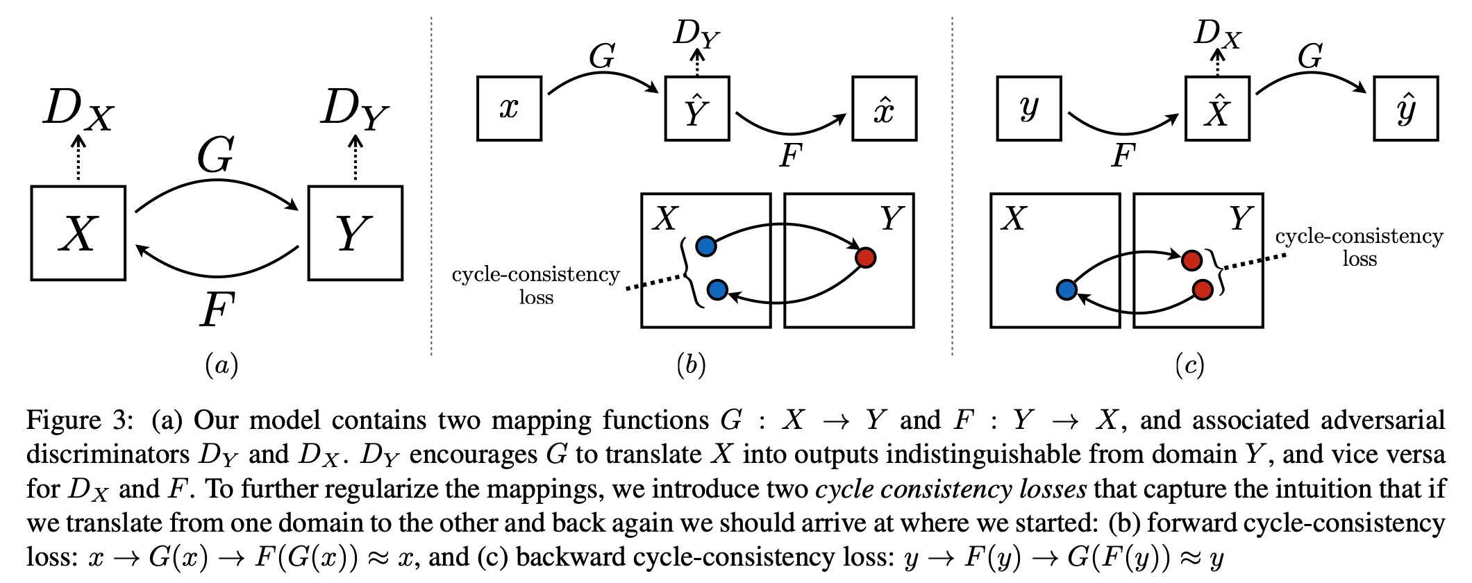
Fig. 39 Learned mappings between source domain \(X\) and target domain \(Y\). Source: [ZPIE17].

Adversarial Loss function, to be minimized by \(G\) and \(F\) and to be maximized by \(D_Y\) and \(D_X\), respectively:

\[\begin{split} L_{adv}(G,D_y,X,Y) & = & \frac{1}{m} \sum\limits_{i=1}^m \log(D_Y(y)) + \frac{1}{m} \sum\limits_{i=1}^m \log(1-D_y(G(x_i))) \\ L_{adv}(F,D_x,Y,X) & = & \frac{1}{m} \sum\limits_{i=1}^m \log(D_X(x)) + \frac{1}{m} \sum\limits_{i=1}^m \log(1-D_x(F(y_i))) \end{split}\]

• The Generator \(G\) is trained, such that it converts \(x\) to something that the Discriminator \(D_y\) can not distinguish from \(y\).

• The Generator \(F\) is trained, such that it converts \(y\) to something that the Discriminator \(D_x\) can not distinguish from \(x\).

Cycle Consitency Loss:

The cycle consistency loss enforces the requirement, that if an input-image is converted to the other domain and back again, by feeding it through both generators, the result should be similar to the input-image.

The minimization of \(L_{cyc}(G,F,X,Y)\) enforces that \(F(G(x)) \approx x\) and \(G(F(y)) \approx y\).

\[ L_{cyc}(G,F,X,Y) = \frac{1}{m} \sum\limits_{i=1}^m || F(G(x_i))-x_i ||_1 + || G(F(y_i))-y_i) ||_1 . \]

Overall Loss-Function:

\[ L_{full} = L_{adv}(G,D_y,X,Y) + L_{adv}(F,D_x,Y,X) + L_{cyc}(G,F,X,Y) \]

Architecture of the Generators \(G\) and \(F\):

Fig. 40 Source: towards data science.

Architecture of the Discriminators \(D_x\) and \(D_y\):

Fig. 41 Source: towards data science.

Cycle GAN Strengths and Limitations:

Cycle GAN works well on tasks, which involve color- or texture-changes, e.g. day-to-night translations, photo-to-painting transformation or style transfer. This can be seen e.g. in this video on Cityscape to GTA5-Style transfer or this video on day- to night-drive transformation.

However, Cycle GAN often fails for tasks, that require substantial geometric changes, as can be seen in the image below.

Fig. 42 Source: [ZPIE17].

Star GAN: Multi-domain transformations

Fig. 43 Example: Transformations between multiple domains. Source: [CCK+18].

In Cycle GAN transformations from a source domain \(X\) to a target domain \(Y\) has been addressed. For transformations between multiple domains, Cycle GAN can also be applied, as shown in image Comparison between Cycle- and Star-GAN for multi-domain transformations. However, in this case for each possible pair of domains an individual Generator pair has to be trained. With Star GAN transformations between multiple domains can be realized using only a single Generator.

Fig. 44 Source: [CCK+18].

Fig. 45 Source: [CCK+18].

Adversarial Loss:

Discriminator \(D\) tries to maximize \(L_{adv}\), whereas the Generator \(G\) tries to minimize it.

\[ L_{adv}= E_x \left[ \log(D_{src}(x)) \right] + E_{x,c} \left[ log(1-D_{src}(G(x,c))) \right], \]

with

• \(x\) real image

• \(c\) label of target domain

• \(D_{src}\) the part of the discriminator which distinguishes real from fake

Domain Classification Loss:

The Domain classification loss of real images to be minimized by \(D\) is:

\[ L_{cls}^r= E_{x,c'} \left[ - \log(D_{cls}(c'|x)) \right]. \]

By minimizing this objective, \(D\) learns to classify a real image \(x\) to its corresponding original domain \(c′\).

The domain classification loss of fake images to be minimized by \(G\) is:

\[ L_{cls}^f= E_{x,c} \left[ - \log(D_{cls}(c|G(x,c))) \right], \]

\(G\) tries to minimize this objective to generate images that can be classified as the target domain \(c\). with

• \(x\) real image

• \(c\) label of target domain

• \(c'\) label of original domain

• \(D_{cls}\) the part of the discriminator which assigns images to corresponding labels.

Reconstruction Loss:

By minimizing the adversarial and classification losses, \(G\) is trained to generate images that are realistic and classified to its correct target domain. However, minimizing the losses does not guarantee that translated images preserve the content of its input images while changing only the domain-related part of the inputs. This problem is alleviated by the reconstruction loss, which is similar to the cycle consistency loss in Cycle GAN.

\[ L_{rec}= E_{x,c',c} \left[ || x - G(G(x,c),c') ||_1 \right], \]

with

• \(x\) real image

• \(c\) label of target domain

• \(c'\) label of original domain

Overall Loss:

Discriminator minimizes

\[ L_D=-L_{adv}+\lambda_{cls} L_{cls}^r. \]

Generator minimizes

\[ L_G=L_{adv}+\lambda_{cls} L_{cls}^f + \lambda_{rec} L_{rec}. \]

Fig. 46 Source: [CCK+18].

Architecture of Star GAN Generator:

The Generator archictecture is similar to the one used in Cycle GAN:

Fig. 47 Source: [CCK+18].

Architecture of Star GAN Discriminator:

The Discriminator \(D\) classifies per patch. For this a Fully Convolutional Neural Network, like in PatchGAN is applied:

Fig. 48 Source: [CCK+18].

Final Remark on Fully Convolutional Network:

In a Fully Convolutional Network (FCNN) dense layers at the output are replaced by convolutional layers, by rearranging the neurons in the dense layer into the channel-dimension of a convolutional layer. In this way images of variable size can be passed to the network and the corresponding output has also a variable size. Each output neuron belongs to one region in the image.

Fig. 49 Neurons of the dense layer are rearranged into channels of a convolutional layer. Since a convolutional layer always has the same number of weights, independent of the size of it’s input, it can manage different sizes of input. In dense layers the number of weights depends on the size of the input. Therefore, dense layers can not cope with variable-size input.