Implementing Neural Networks with Keras
Contents
Implementing Neural Networks with Keras#
Author: Johannes Maucher
Last Update: 29.11.2022
What you will learn:#
Define, train and evaluate MLP in Keras
Define, train and evaluate CNN in Keras
Visualization of learning-curves
Implement cross-validation in Keras
Image classification based on the CIFAR-10 dataset, which is included in Keras datasets.
Imports and Configurations#
#!pip install visualkeras
#!pip install Pillow
#!pip install tensorflow-cpu
#import tensorflow
#from tensorflow import keras
from matplotlib import pyplot as plt
import numpy as np
from tensorflow.keras.datasets import cifar10
from tensorflow.keras.models import Sequential, Model, load_model
from tensorflow.keras.layers import Dense,Input,Dropout,Flatten,Conv2D,MaxPool2D
from tensorflow.keras.optimizers import SGD
from tensorflow.keras.utils import to_categorical
from tensorflow.keras.backend import set_image_data_format
import os
set_image_data_format("channels_last")
import warnings
warnings.filterwarnings("ignore")
The following code-cell is just relevant if notebook is executed on a computer with multiple GPUs. It allows to select the GPU.
#from os import environ
#environ["CUDA_DEVICE_ORDER"]="PCI_BUS_ID"
#environ["CUDA_VISIBLE_DEVICES"]="1"
In this notebook the neural network shall not learn models, which already exists. This is implemented as follows. The three models (MLP and two different CNNs) are saved to the files, whose name is assigned to the variables mlpmodelname, cnnsimplemodelname and cnnadvancedmodelname, respectively.
If these files exist (checked by os.path.isfile(filename)) a corresponding AVAILABLE-Flag is set. If this flag is False, the corresponding model will be learned and saved, otherwise the existing model will be loaded from disc.
modeldirectory="models/"
mlpmodelname=modeldirectory+"dense512"
cnnsimplemodelname=modeldirectory+"2conv32-dense512"
cnnadvancedmodelname=modeldirectory+"2conv32-4conv64-dense512"
import os.path

if os.path.isdir(mlpmodelname):
    MLP_AVAILABLE=True
else:
    MLP_AVAILABLE=False

if os.path.isdir(cnnsimplemodelname):
    CNN1_AVAILABLE=True
else:
    CNN1_AVAILABLE=False

if os.path.isdir(cnnadvancedmodelname):
    CNN2_AVAILABLE=True
else:
    CNN2_AVAILABLE=False
CNN1_AVAILABLE
False
Access Data#
Load the Cifar10 image dataset from keras.datasets. Determine the shape of the training- and the test-partition.
(X_train, y_train), (X_test, y_test) = cifar10.load_data()
print(np.shape(X_train))
print(np.shape(X_test))
(50000, 32, 32, 3)
(10000, 32, 32, 3)
Visualize Data#
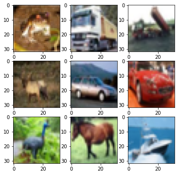
Viusalize the first 9 images of the training-partition, using function imshow() from matplotlib.pyplot.
# create a grid of 3x3 images
plt.figure(figsize=(6,6))
for i in range(9):
    plt.subplot(3,3,i+1)
    B=X_train[i].copy()
    #B=B.swapaxes(0,2)
    #B=B.swapaxes(0,1)
    plt.imshow(B)
# show the plot
plt.show()
Preprocessing#
Scale all images such that all their values are in the range \([0,1]\).
X_train = X_train.astype('float32')
X_test = X_test.astype('float32')
X_train = X_train / 255.0
X_test = X_test / 255.0
Labels of the first 9 training images:
print(y_train[:9])
[[6]
 [9]
 [9]
 [4]
 [1]
 [1]
 [2]
 [7]
 [8]]
Label-Encoding: Transform the labels of the train- and test-partition into a one-hot-encoded representation.
y_train=to_categorical(y_train)
y_test=to_categorical(y_test)
num_classes=len(y_train[0,:])
print(y_train[:9,:])
[[0. 0. 0. 0. 0. 0. 1. 0. 0. 0.]
 [0. 0. 0. 0. 0. 0. 0. 0. 0. 1.]
 [0. 0. 0. 0. 0. 0. 0. 0. 0. 1.]
 [0. 0. 0. 0. 1. 0. 0. 0. 0. 0.]
 [0. 1. 0. 0. 0. 0. 0. 0. 0. 0.]
 [0. 1. 0. 0. 0. 0. 0. 0. 0. 0.]
 [0. 0. 1. 0. 0. 0. 0. 0. 0. 0.]
 [0. 0. 0. 0. 0. 0. 0. 1. 0. 0.]
 [0. 0. 0. 0. 0. 0. 0. 0. 1. 0.]]
MLP#
Architecture#
In Keras the architecture of neural networks can be defined in two different ways:
Using the
SequentialmodelUsing the functional API
Below the two approaches are demonstrated. The first approach is simpler, but restricted to neural networks which consist of a linear stack of layers. The second approach is more flexible and allows to define quit complex network architectures, e.g. with more than one input, more than one output or with parallel branches.
Network definition option1: Using the sequential model#
if MLP_AVAILABLE:
model=load_model(mlpmodelname)
print("MLP MODEL ALREADY AVAILABLE \nLOAD EXISTING MODEL")
else:
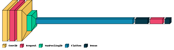
model = Sequential()
model.add(Flatten(input_shape=(32, 32,3)))
model.add(Dense(512, activation='relu'))
model.add(Dense(num_classes, activation='softmax'))
model.summary()
Model: "sequential_4"
_________________________________________________________________
 Layer (type)                Output Shape              Param #
=================================================================
 flatten_5 (Flatten)         (None, 3072)              0

 dense_10 (Dense)            (None, 512)               1573376

 dense_11 (Dense)            (None, 10)                5130

=================================================================
Total params: 1,578,506
Trainable params: 1,578,506
Non-trainable params: 0
_________________________________________________________________
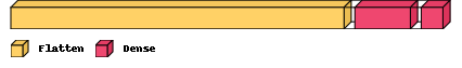
import visualkeras
visualkeras.layered_view(model,legend=True)
Network definition option 2: Using the functional API#
# This returns a tensor
inputs = Input(shape=(32, 32,3))
x=Flatten()(inputs)
x=Dense(512, activation='relu')(x)
x=Dense(num_classes, activation='softmax')(x)
model2 = Model(inputs=inputs, outputs=x)
model2.summary()
Model: "model_1"
_________________________________________________________________
 Layer (type)                Output Shape              Param #
=================================================================
 input_2 (InputLayer)        [(None, 32, 32, 3)]       0

 flatten_6 (Flatten)         (None, 3072)              0

 dense_12 (Dense)            (None, 512)               1573376

 dense_13 (Dense)            (None, 10)                5130

=================================================================
Total params: 1,578,506
Trainable params: 1,578,506
Non-trainable params: 0
_________________________________________________________________
Define Training Parameters#
Apply Stochastic Gradient Descent (SGD) learning, for minimizing the categorical_crossentropy. The performance metric shall be accuracy. Train the network.
if not MLP_AVAILABLE:
    # Compile model
    epochs = 8
    lrate = 0.01
    decay = lrate/epochs
    sgd = SGD(lr=lrate, momentum=0.9, decay=decay)
    model.compile(loss='categorical_crossentropy', optimizer=sgd, metrics=['accuracy'])
Perform Training#
if not MLP_AVAILABLE:
    history=model.fit(X_train, y_train, validation_data=(X_test, y_test), epochs=epochs, batch_size=32,verbose=False)
    model.save(mlpmodelname)
    MLP_AVAILABLE=True
else:
    print("TRAINED MODEL ALREADY AVAILABLE")
INFO:tensorflow:Assets written to: models/dense512/assets
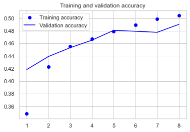
Evaluation#
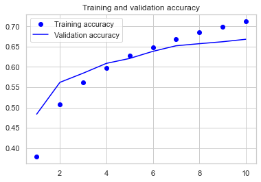
Visualize the learning-curve on training- and test-data.
import matplotlib.pyplot as plt
%matplotlib inline
import seaborn as sb
sb.set_style("whitegrid")
sb.set_context("notebook")
try:
    acc = history.history['accuracy']
    val_acc = history.history['val_accuracy']
    max_val_acc=np.max(val_acc)

    epochs = range(1, len(acc) + 1)

    plt.figure()

    plt.plot(epochs, acc, 'bo', label='Training accuracy')
    plt.plot(epochs, val_acc, 'b', label='Validation accuracy')
    plt.title('Training and validation accuracy')
    plt.legend()
    plt.show()
except:
    print("LEARNING CURVE ONLY AVAILABLE IF TRAINING HAS BEEN PERFORMED IN THIS RUN")
loss,acc = model.evaluate(X_train,y_train, verbose=0)
print("Accuracy on Training Data : %.2f%%" % (acc*100))
Accuracy on Training Data : 51.27%
loss,acc = model.evaluate(X_test,y_test, verbose=0)
print("Accuracy on Test Data: %.2f%%" % (acc*100))
Accuracy on Test Data: 49.03%
CNN#
Define Architecture#
if CNN1_AVAILABLE:
    model=load_model(cnnsimplemodelname)
    print("CNN SIMPLE MODEL ALREADY AVAILABLE \nLOAD EXISTING MODEL")
else:
    model = Sequential()
    model.add(Conv2D(filters=32, kernel_size=(3, 3), input_shape=(32, 32,3), padding='same',activation='relu'))
    model.add(Dropout(0.2))
    model.add(Conv2D(filters=32, kernel_size=(3, 3), activation='relu',padding='same'))
    model.add(MaxPool2D(pool_size=(2, 2)))
    model.add(Flatten())
    model.add(Dense(512, activation='relu'))
    model.add(Dropout(0.5))
    model.add(Dense(num_classes, activation='softmax'))
model.summary()
Model: "sequential_5"
_________________________________________________________________
 Layer (type)                Output Shape              Param #
=================================================================
 conv2d_8 (Conv2D)           (None, 32, 32, 32)        896

 dropout_6 (Dropout)         (None, 32, 32, 32)        0

 conv2d_9 (Conv2D)           (None, 32, 32, 32)        9248

 max_pooling2d_4 (MaxPooling  (None, 16, 16, 32)       0
 2D)

 flatten_7 (Flatten)         (None, 8192)              0

 dense_14 (Dense)            (None, 512)               4194816

 dropout_7 (Dropout)         (None, 512)               0

 dense_15 (Dense)            (None, 10)                5130

=================================================================
Total params: 4,210,090
Trainable params: 4,210,090
Non-trainable params: 0
_________________________________________________________________
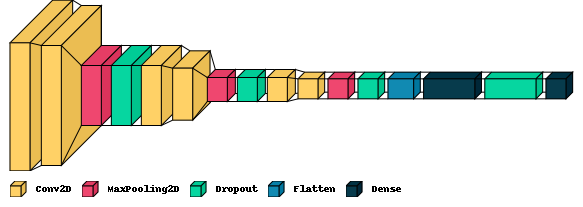
visualkeras.layered_view(model,legend=True)
Define Training Parameters#
if not CNN1_AVAILABLE:
    # Compile model
    epochs = 10
    lrate = 0.01
    decay = lrate/epochs
    sgd = SGD(lr=lrate, momentum=0.9, decay=decay, nesterov=False)
    model.compile(loss='categorical_crossentropy', optimizer=sgd, metrics=['accuracy'])
Perform Training#
if not CNN1_AVAILABLE:
    history=model.fit(X_train, y_train, validation_data=(X_test, y_test), epochs=epochs, batch_size=32)
    model.save(cnnsimplemodelname)
    CNN1_AVAILABLE=True
else:
    print("TRAINED MODEL ALREADY AVAILABLE")
Epoch 1/10
1563/1563 [==============================] - 59s 38ms/step - loss: 1.7212 - accuracy: 0.3783 - val_loss: 1.4325 - val_accuracy: 0.4836
Epoch 2/10
1563/1563 [==============================] - 63s 41ms/step - loss: 1.3712 - accuracy: 0.5078 - val_loss: 1.2339 - val_accuracy: 0.5620
Epoch 3/10
1563/1563 [==============================] - 63s 41ms/step - loss: 1.2190 - accuracy: 0.5621 - val_loss: 1.1625 - val_accuracy: 0.5846
Epoch 4/10
1563/1563 [==============================] - 66s 42ms/step - loss: 1.1282 - accuracy: 0.5976 - val_loss: 1.1109 - val_accuracy: 0.6088
Epoch 5/10
1563/1563 [==============================] - 67s 43ms/step - loss: 1.0471 - accuracy: 0.6281 - val_loss: 1.0784 - val_accuracy: 0.6209
Epoch 6/10
1563/1563 [==============================] - 70s 45ms/step - loss: 0.9900 - accuracy: 0.6475 - val_loss: 1.0306 - val_accuracy: 0.6384
Epoch 7/10
1563/1563 [==============================] - 71s 45ms/step - loss: 0.9353 - accuracy: 0.6691 - val_loss: 0.9897 - val_accuracy: 0.6522
Epoch 8/10
1563/1563 [==============================] - 73s 47ms/step - loss: 0.8946 - accuracy: 0.6849 - val_loss: 0.9800 - val_accuracy: 0.6573
Epoch 9/10
1563/1563 [==============================] - 75s 48ms/step - loss: 0.8538 - accuracy: 0.6992 - val_loss: 0.9672 - val_accuracy: 0.6621
Epoch 10/10
1563/1563 [==============================] - 74s 47ms/step - loss: 0.8136 - accuracy: 0.7130 - val_loss: 0.9564 - val_accuracy: 0.6682
WARNING:absl:Found untraced functions such as _jit_compiled_convolution_op, _jit_compiled_convolution_op while saving (showing 2 of 2). These functions will not be directly callable after loading.
INFO:tensorflow:Assets written to: models/2conv32-dense512/assets
INFO:tensorflow:Assets written to: models/2conv32-dense512/assets
Evaluation#
try:
    acc = history.history['accuracy']
    val_acc = history.history['val_accuracy']
    max_val_acc=np.max(val_acc)

    epochs = range(1, len(acc) + 1)

    plt.figure()

    plt.plot(epochs, acc, 'bo', label='Training accuracy')
    plt.plot(epochs, val_acc, 'b', label='Validation accuracy')
    plt.title('Training and validation accuracy')
    plt.legend()
    plt.show()
except:
    print("LEARNING CURVE ONLY AVAILABLE IF TRAINING HAS BEEN PERFORMED IN THIS RUN")
loss,acc = model.evaluate(X_train,y_train, verbose=0)
print("Accuracy on Training Data : %.2f%%" % (acc*100))
Accuracy on Training Data : 78.31%
loss,acc = model.evaluate(X_test, y_test, verbose=0)
print("Accuracy on Test Data: %.2f%%" % (acc*100))
Accuracy on Test Data: 66.82%
A more complex CNN#
Architecture#
def createModel():
    model = Sequential()
    # The first two layers with 32 filters of window size 3x3
    model.add(Conv2D(32, (3, 3), padding='same', activation='relu', input_shape=(32, 32,3)))
    model.add(Conv2D(32, (3, 3), activation='relu'))
    model.add(MaxPool2D(pool_size=(2, 2)))
    model.add(Dropout(0.25))

    model.add(Conv2D(64, (3, 3), padding='same', activation='relu'))
    model.add(Conv2D(64, (3, 3), activation='relu'))
    model.add(MaxPool2D(pool_size=(2, 2)))
    model.add(Dropout(0.25))

    model.add(Conv2D(64, (3, 3), padding='same', activation='relu'))
    model.add(Conv2D(64, (3, 3), activation='relu'))
    model.add(MaxPool2D(pool_size=(2, 2)))
    model.add(Dropout(0.25))

    model.add(Flatten())
    model.add(Dense(512, activation='relu'))
    model.add(Dropout(0.5))
    model.add(Dense(num_classes, activation='softmax'))

    return model
if CNN2_AVAILABLE:
    model=load_model(cnnadvancedmodelname)
    print("CNN ADVANCED MODEL ALREADY AVAILABLE \nLOAD EXISTING MODEL")
else:
    model = createModel()
model.summary()
Model: "sequential_6"
_________________________________________________________________
 Layer (type)                Output Shape              Param #
=================================================================
 conv2d_10 (Conv2D)          (None, 32, 32, 32)        896

 conv2d_11 (Conv2D)          (None, 30, 30, 32)        9248

 max_pooling2d_5 (MaxPooling  (None, 15, 15, 32)       0
 2D)

 dropout_8 (Dropout)         (None, 15, 15, 32)        0

 conv2d_12 (Conv2D)          (None, 15, 15, 64)        18496

 conv2d_13 (Conv2D)          (None, 13, 13, 64)        36928

 max_pooling2d_6 (MaxPooling  (None, 6, 6, 64)         0
 2D)

 dropout_9 (Dropout)         (None, 6, 6, 64)          0

 conv2d_14 (Conv2D)          (None, 6, 6, 64)          36928

 conv2d_15 (Conv2D)          (None, 4, 4, 64)          36928

 max_pooling2d_7 (MaxPooling  (None, 2, 2, 64)         0
 2D)

 dropout_10 (Dropout)        (None, 2, 2, 64)          0

 flatten_8 (Flatten)         (None, 256)               0

 dense_16 (Dense)            (None, 512)               131584

 dropout_11 (Dropout)        (None, 512)               0

 dense_17 (Dense)            (None, 10)                5130

=================================================================
Total params: 276,138
Trainable params: 276,138
Non-trainable params: 0
_________________________________________________________________
visualkeras.layered_view(model,legend=True)
Define Training Parameters#
if not CNN2_AVAILABLE:
    batch_size = 256
    epochs = 50
    model.compile(optimizer='rmsprop', loss='categorical_crossentropy', metrics=['accuracy'])
Perform Training#
if not CNN2_AVAILABLE:
    history = model.fit(X_train, y_train, batch_size=batch_size, epochs=epochs, verbose=0, validation_data=(X_test, y_test))
    model.save(cnnadvancedmodelname)
    CNN2_AVAILABLE=True
else:
    print("TRAINED MODEL ALREADY AVAILABLE")
WARNING:absl:Found untraced functions such as _jit_compiled_convolution_op, _jit_compiled_convolution_op, _jit_compiled_convolution_op, _jit_compiled_convolution_op, _jit_compiled_convolution_op while saving (showing 5 of 6). These functions will not be directly callable after loading.
INFO:tensorflow:Assets written to: models/2conv32-4conv64-dense512/assets
INFO:tensorflow:Assets written to: models/2conv32-4conv64-dense512/assets
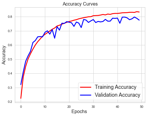
Evaluate#
try:
    plt.figure(figsize=[8,6])
    plt.plot(history.history['accuracy'],'r',linewidth=3.0)
    plt.plot(history.history['val_accuracy'],'b',linewidth=3.0)
    plt.legend(['Training Accuracy', 'Validation Accuracy'],fontsize=18)
    plt.xlabel('Epochs ',fontsize=16)
    plt.ylabel('Accuracy',fontsize=16)
    plt.title('Accuracy Curves',fontsize=16)
    plt.show()
except:
    print("LEARNING CURVE ONLY AVAILABLE IF TRAINING HAS BEEN PERFORMED IN THIS RUN")
loss,acc = model.evaluate(X_train,y_train, verbose=0)
print("Accuracy on Training Data : %.2f%%" % (acc*100))
Accuracy on Training Data : 86.97%
loss,acc = model.evaluate(X_test,y_test, verbose=0)
print("Accuracy on Test Data : %.2f%%" % (acc*100))
Accuracy on Test Data : 77.59%
Visualize Feature Maps in 2nd Conv-Layer#
The output of an arbitrary layer, for a given input image can be visualized as demonstrated below.
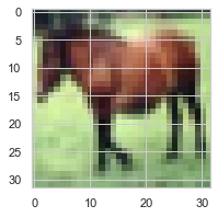
First we select and display an image, for which the featuremaps in the 2nd Convolution Layer of the previously defined and trained network shall be generated:
img=X_train[7:8,:,:,:]
img.shape
(1, 32, 32, 3)
plt.figure(figsize=(3,3))
plt.imshow(img[0])
<matplotlib.image.AxesImage at 0x7fb15238a880>
Next, we define a network, which contains the first 2 convolution layers of the previously trained network:
FirstLayer=Model(inputs=model.inputs, outputs=model.layers[1].output)
FirstLayer.summary()
Model: "model_16"
_________________________________________________________________
 Layer (type)                Output Shape              Param #
=================================================================
 conv2d_10_input (InputLayer  [(None, 32, 32, 3)]      0
 )

 conv2d_10 (Conv2D)          (None, 32, 32, 32)        896

 conv2d_11 (Conv2D)          (None, 30, 30, 32)        9248

=================================================================
Total params: 10,144
Trainable params: 10,144
Non-trainable params: 0
_________________________________________________________________
Then we pass the selected image to the extracted subnetwork. The output are the feature-maps of the second convolutional layer:
feature_maps = FirstLayer.predict(img)
1/1 [==============================] - 0s 28ms/step
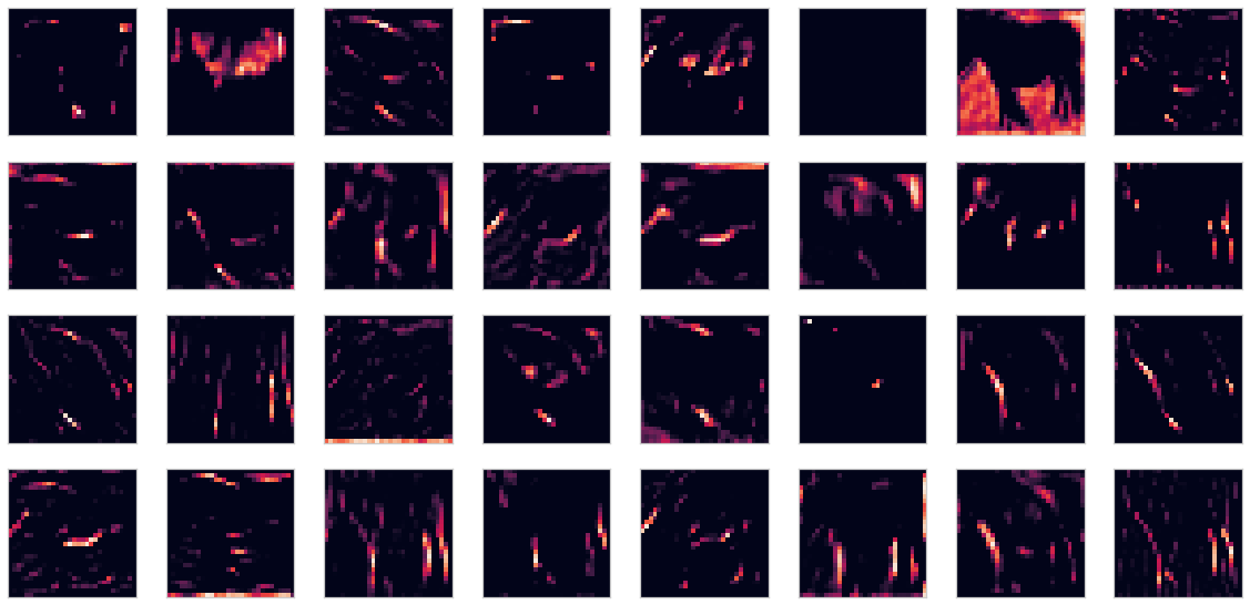
There are 32 feature-maps, each of size \((32 \times 32)\):
feature_maps.shape
(1, 30, 30, 32)
Finally we visualize these 32 feature-maps:
square = 8
ix = 1
plt.figure(figsize=(20,20))
for _ in range(8):
    for _ in range(4):
        ax = plt.subplot(square, square, ix)
        ax.set_xticks([])
        ax.set_yticks([])
        plt.imshow(feature_maps[0, :, :, ix-1])
        ix += 1
plt.show()