Linear Regression

For a given set of labeled training data

\[ T=\{\mathbf{x}_t,r_t \}_{t=1}^N, \]

where the targets \(r_t\) are numeric values, usually from \(\mathcal{R}\) and the inputs \(\mathbf{x}_t=(x_{1,t}, \ldots, x_{d,t})\) are numeric vectors of length \(d\), the goal of regression is to learn a function, which maps the input-vectors to the target-values.

We usually assume that the targets \(r\) can be calculated as a sum of a determinisitc function \(f(\mathbf{x})\) and a non-determininstic noise \(n\)

\[ r=f(\mathbf{x})+n, \]

and we like to find a good approximation \(g(\mathbf{x}|\Theta)\) for the unknown deterministic part \(f(\mathbf{x})\).

In linear regression we assume that the approximation \(g(x|\Theta)\) is a linear function of type

(1)\[ g(\mathbf{x})=w_0 + w_1 x_1 + w_2 x_2 + \cdots + w_d x_d \]

This means, that we assume a certain type of function and we want to learn the parameters

\[ \Theta = \lbrace w_0, w_1, \ldots , w_d \rbrace \]

from data, such that the corresponding \(g(\mathbf{x}|\Theta)\) is a good estimate for \(f(\mathbf{x})\).

Concerning the non-deterministic part \(n\) one often assumes that it is a Gaussian-distributed random variable of mean \(\mu=0\) and standard-deviation \(\sigma\). In this case the posterior \(p(r|\mathbf{x})\) is also a Gaussian distribution with standard-deviation \(\sigma\) and mean \(\mu=g(\mathbf{x} \mid \theta)\).

Maximum-Likelihood Estimation

Maximum-Likelihood Estimation (MLE) estimates the parameters \(\Theta\), such that the corresponding \(g(\mathbf{x}|\Theta)\) is the one, which most likely generates the given set of training data \(T\).

Under the assumption that noise \(n\) is a Gaussian-distributed variable of mean \(\mu=0\), one can prove that the MLE approach can be realized by minimizing the Sum of Squared Error (SSE) Loss function:

(2)\[ E(\Theta | T)=\frac{1}{2} \sum\limits_{t=1}^N [r_t-g(\mathbf{x}_t|\Theta)]^2 = \frac{1}{2} \sum\limits_{t=1}^N [r_t-(w_0 + w_1 x_{1,t} + \cdots + w_d x_{d,t})]^2 \]

This means that the learning task is: Determine the parameters \(w_i \in \Theta\), which minimize the SSE (function (2)).

In general, in order to find the value \(x\), at which a function \(f(x)\) is minimal, we have to calculate the first derivation \(f'(x)=\frac{\partial f}{\partial x} \) and determine it’s zeros.

Here we have an error function \(E(\Theta | T)\), which depends not only on a single variable, but on all weights \(w_i \in \Theta\). Hence, we have to determine all partial derivatives

\[\begin{split} \frac{\partial E}{\partial w_0} &=& \sum\limits_{t=1}^N \left[r_t-(w_0 + w_1 x_{1,t} + \cdots + w_d x_{d,t})\right] \cdot -1 \\ \frac{\partial E}{\partial w_1} &=& \sum\limits_{t=1}^N \left[r_t-(w_0 + w_1 x_{1,t} + \cdots + w_d x_{d,t})\right] \cdot -x_{1,t} \\ \vdots &=& \vdots \nonumber \\ \frac{\partial E}{\partial w_d} &=& \sum\limits_{t=1}^N \left[r_t-(w_0 + w_1 x_{1,t} + \cdots + w_d x_{d,t})\right] \cdot -x_{d,t} \end{split}\]

and set them equal to zero. This yields a system of \(d+1\) linear equations, which can be written as a matrix-multiplication

(3)\[ \mathbf{y}=\mathbf{A} \cdot \mathbf{w}, \]

and solving for \(\mathbf{w}\) yields:

(4)\[ \mathbf{w} = \mathbf{A}^{-1} \mathbf{y}, \]

where

\[\begin{split} \mathbf{A}= \left[ \begin{array}{ccccc} N & \sum\limits_{t=1}^N x_{1,t} & \sum\limits_{t=1}^N x_{2,t} & \cdots & \sum\limits_{t=1}^N x_{d,t}\\ \sum\limits_{t=1}^N x_{1,t} & \sum\limits_{t=1}^N x_{1,t} x_{1,t} & \sum\limits_{t=1}^N x_{1,t} x_{2,t}& \cdots & \sum\limits_{t=1}^N x_{1,t} x_{d,t} \\ \vdots & \vdots & \vdots & \vdots & \vdots \\ \sum\limits_{t=1}^N x_{d,t} & \sum\limits_{t=1}^N x_{d,t} x_{1,t} & \sum\limits_{t=1}^N x_{d,t} x_{2,t} & \cdots & \sum\limits_{t=1}^N x_{d,t} x_{d,t} \\ \end{array} \right], \qquad \mathbf{w} = \left[ \begin{array}{c} w_0 \\ w_1 \\ \vdots \\ w_d \end{array} \right], \qquad \mathbf{y} = \left[ \begin{array}{c} \sum\limits_{t=1}^N r_t \\ \sum\limits_{t=1}^N r_t x_{1,t} \\ \vdots \\ \sum\limits_{t=1}^N r_t x_{d,t}\\ \end{array} \right] \end{split}\]

For an efficient solution one usually calulates \(\mathbf{A}\) and \(\mathbf{y}\) as follows:

\[\begin{split} \mathbf{A} & = & \mathbf{D}^T \mathbf{D} \nonumber \\ \mathbf{y} & = & \mathbf{D}^T \mathbf{r} \nonumber \end{split}\]

where

\[\begin{split} \mathbf{D}= \left[ \begin{array}{ccccc} 1 & x_{1,1} & x_{2,1} & \cdots & x_{d,1} \\ 1 & x_{1,2} & x_{2,2} & \cdots & x_{d,2} \\ \vdots & \vdots & \vdots & \vdots & \vdots \\ 1 & x_{1,N} & x_{2,N} & \cdots & x_{d,N} \\ \end{array} \right] \qquad \mbox{and} \qquad \mathbf{r} = \left[ \begin{array}{c} r_1 \\ r_2 \\ \vdots \\ r_N \\ \end{array} \right] \end{split}\]

By expressing \(\mathbf{A}\) and \(\mathbf{y}\) in eauation (4) in terms of \(\mathbf{D}\) and \(\mathbf{r}\) the weights, which minimize the loss function are:

(5)\[ \mathbf{w}= \left( \mathbf{D}^T \mathbf{D} \right)^{-1} \mathbf{D}^T \mathbf{r}. \]

Note

The approach described above is a quite old type of linear regression. In the literature it is often called Ordinary Least Square (OLS). In scikit-learn the name of the corresponding OLS-module is just LinearRegression

Generalized Linear Regression

With Linear Regression one can not only learn linear functions \(g(\mathbf{x})\) of type (1). Since we are free to preprocess the input vectors \(\mathbf{x}\) with an arbitrary aomount \(z\) of preprocessing functions \(\Phi_i\) of arbitrary type (linear and non-linear), a Generlized Linear Regression of type

(6)\[ g(\mathbf{x})=w_0 + w_1 \Phi_1(\mathbf{x}) + w_2 \Phi_2(\mathbf{x}) + \cdots + w_z \Phi_z(\mathbf{x}) \]

can be learned. Note that this is still called linear regression, because we are still linear in the variable’s \(w_i\).

Example Generalized Linear Regression with

Assume that the input vectors are of dimension \(d=2\), i.e. \(\mathbf{x}=(x_1,x_2)\) and we like to learn a quadratic function. For this we can define a set of functions \(\Phi_i\):

(7)\[\begin{split} \Phi_1(\mathbf{x}) & = & x_1 \\ \Phi_2(\mathbf{x}) & = & x_2 \\ \Phi_3(\mathbf{x})& = & x_1 x_2 \\ \Phi_5(\mathbf{x}) & = & x_1^2 \\ \Phi_6(\mathbf{x}) &=& x_2^2 \end{split}\]

The learning task is then to determine the weights \(w_i\) of the polynomial

(8)\[ g(\mathbf{x})=w_0 + w_1 \Phi_1(\mathbf{x}) + w_2 \Phi_2(\mathbf{x} + \cdots + w_6 \Phi_6(\mathbf{x}) \]

which yields the minimum loss.

Finding the weights \(w_i\), which minimize the loss function, can be performed in the same way as described above. One just has to replace all \(x_{i,t}\) by \(\Phi_i(\mathbf{x}_t)\). In particular \(\mathbf{w}\) can be calculated as in equation (5), but now matrix \(D\) is

(9)\[\begin{split} \mathbf{D}= \left[ \begin{array}{ccccc} 1 & \Phi_1(\mathbf{x}_{1}) & \Phi_2(\mathbf{x}_{1})& \cdots & \Phi_z(\mathbf{x}_{1}) \\ 1 & \Phi_1(\mathbf{x}_{2}) & \Phi_2(\mathbf{x}_{2})& \cdots & \Phi_z(\mathbf{x}_{2}) \\ \vdots & \vdots & \vdots & \vdots & \vdots \\ 1 & \Phi_1(\mathbf{x}_{N}) & \Phi_2(\mathbf{x}_{N})& \cdots & \Phi_z(\mathbf{x}_{N}) \\ \end{array} \right] \end{split}\]

Regularisation

In Machine Learning Regularisation is a technique to avoid overfitting. With regularisation the weights are learned such that they not only minimize a loss function on training data (e.g. the Mean Squared Error) but simultaneously have as low as possible absolut values. This additional restriction - absolute values of weights shall be low - yields better generalisation because functions with lower coefficients \(w_i\) are smoother. However, the challenge is to find a good trade-off between minimizing the error on training data and minimizing the weights \(w_i\). If too much emphasis is put on the weight-minimizsation the learned function may be to simple, i.e. it is underfitted to training data.

The different regularisation methods, described below, learn weights by minimizing training-error and a regularisation term simultaneously:

(10)\[ weights = argmin\left( E(w,T) + \lambda \cdot regularisationterm(w) \right) \]

The different techniques described below all perform linear regression, but differ in the used regularisation-term. The hyperparameter \(\lambda\) is used to control the trade-off between error-minimisation and weight-minimisation.

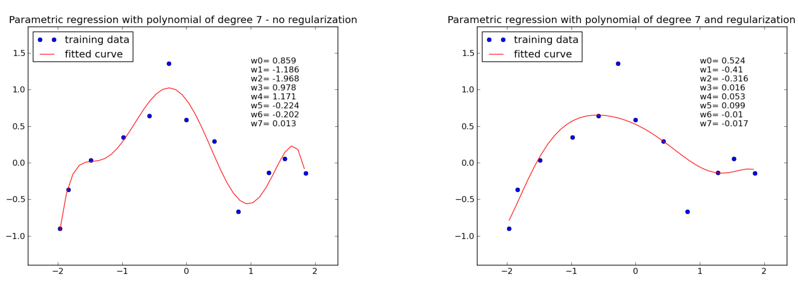
Fig. 1 The plot on the left hand side displays a polynomial of degree 7, which has been learned from the given training data without regularisation. It can be observed, that the weights have comparatively high values and the learned function is tightly fitted to training data (overfitted). In contrast on the right hand side regularisation has been applied (Ridge regression). It can be seen, that now the learned weights are much smaller and the corresponding curve is smoother and not overfitted to training data.

Ridge Regression

In Ridge-Regression the error-function \(E(w,T)\) in equation (10) is the MSE and the regularisation term is the squared L2-norm. I.e. Ridge-Regression minimizes

(11)\[ \mathbf{w}=argmin\left( \sum\limits_{t=1}^N [r_t-g(\mathbf{x}_t|\Theta)]^2 + \lambda \cdot ||w||_2^2 \right), \]

where the p-norm \(||w||_p\) is defined to be

(12)\[ ||w||_p = \left(\sum\limits_{i} |w_i|^p \right)^{\frac{1}{p}} \]

For Ridge Regression, scikit-learn provides the class Ridge.

Lasso

Lasso regularisation provides sparse weights. This means that many weights are zero or very close to zero and only the weights which belong to the most important features are non-zero. This sparsity can be achieved by applying the L1-Norm as regularisation term.

(13)\[ \mathbf{w}=argmin\left( \sum\limits_{t=1}^N [r_t-g(\mathbf{x}_t|\Theta)]^2 + \lambda \cdot ||w||_1 \right), \]

For Lasso Regression, scikit-learn provides the class Lasso.

Elastic-Net

Elastic-Net regularisation applies a regularisation term, which is a weighted sum of L1- and L2-norm.

(14)\[ \mathbf{w}=argmin\left( \sum\limits_{t=1}^N [r_t-g(\mathbf{x}_t|\Theta)]^2 + \lambda \rho ||w||_1 + \frac{\lambda (1-\rho)}{2} ||w||_2^2 \right), \]

For Elastic-Net Regression, scikit-learn provides the class ElasticNet.