Sequence-To-Sequence, Attention, Transformer

Sequence-To-Sequence

In the context of Machine Learning a sequence is an ordered data structure, whose successive elements are somehow correlated.

Examples:

• Univariate Time Series Data:

  • Stock price of a company

  • Average daily temperature over a certain period of time

  • In general data which is tracked by sensors over time, e.g. accelaration, speed, energy-consuption, pressure, emissions, …

• Multivariate Time Series Data:

  • For a specific product in an online-shop: Daily number of clicks, number of purchases, number of ratings, number of returns

• Natural Language: The words in a sentence, section, article, …

• Image: Sequence of pixels

• Video: Sequence of frames

The crucial property of sequences is the correlation between the individual datapoints. This means that for each element (datapoint) of the sequence, information is not only provided by it’s individual feature-vector, but also by the neighboring datapoints. For each element of the sequence, the neighboring elements are called context and we can understand an individual element by taking in account

• it’s feature vector

• the contextual information, provided by the neighbours

An example of how the human brain exploits context-information in order to recognize is given in the image below.

Fig. 78 Understand by integration of contextual information.

For all types of sequential data, Machine Learning algorithms should learn models, which regard not only individual feature vectors, but also contextual information. For example Recurrent Networks (RNN) are capable to do so. In this section more complex ML architectures, suitable for sequential data will be described. Some of these architectures integrate Recurrent Neural Networks. More recent architectures, Transformers, integrate the concept of Attention. Both, Attention and the integration of Attention in Transformers will be described in this section.

As already mentioned in section Recurrent Networks (RNN), ML algorithms, which take sequential data at their input, either output one element per sequence (many-to-one) or a sequence of elements (many-to-many). The latter is the same as Sequence-To-Sequence learning.

Sequence-To-Sequence (Seq2Seq) models ([CvMG+14], [SVL14]) map

• input sequences \(\mathbf{x}=(x_1,x_2,\ldots x_{T_x})\)

• to output sequences \(\mathbf{y}=(y_1,y_2,\ldots y_{T_y})\)

The lengths of input- and output sequence need not be the same.

Applications of Seq2Seq models are e.g. Language Models (LM) or Machine Translation.

Simple Architecture for aligned Sequences

The simplest architecture for a Sequence-To-Sequence consists of an input layer, an RNN layer and a Dense layer (with a softmax activation). Such an architecture is depicted in the time-unfolded representation in figure Simple architecture for aligned sequences.

The hidden states \(h_i\) are calculated by

\[ h_{i} = f(x_i,h_{i-1}) \quad \forall i \in [1,T], \]

where the function \(f()\) is realized by a Vanilla RNN, LSTM, GRU. The Dense layer at the output realizes the function

\[ y_i = g(h_i) \quad \forall i \in [1,T]. \]

If the Dense layer at the output has a softmax-activation, and the architecture is trained to predict the next token in the sequence, the output at each time step \(t\) is the conditional distribution

\[ p(x_t \mid x_{t-1}, \ldots , x_1). \]

In this way a language model can be implemented. Language models allow to predict a target word from the context words (neighbouring words).

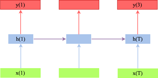
Fig. 79 Simple Seq2Seq architecture for alligned input- and output sequence. The input-sequence is processed (green) by a Recurrent Neural layer (Vanilla RNN, LSTM, GRU, etc.) and the hidden states (blue) at the output of the Recurrent layer are passed to a dense layer with softmax-activation. The output sequence (red) is alligned to the input sequence in the sense that each \(y_i\) corresponds to \(x_i\). This also implies that both sequences have the same length.

Encoder-Decoder Architectures

In an Encoder-Decoder architecture, the Encoder maps the input sequence \(\mathbf{x}=(x_1,x_2,\ldots x_{T_x})\) to an intermediate representation, also called context vector, \(\mathbf{c}\). The entire information of the sequences is compressed in this vector. The context vector is applied as input to the Decoder, which outputs a sequence \(\mathbf{y}=(y_1,y_2,\ldots y_{T_y})\). With this architecture the input- and output-sequence need not be alligned.

There exists a phletora of different Seq2Seq Encoder-Decoder architectures. Here, we first refer to one of the first architectures, introduced by Cho et al in [CvMG+14].

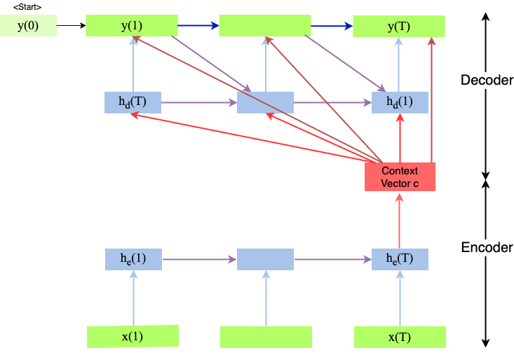
Fig. 80 Seq2Seq Architecture as introduced in [CvMG+14]. Applicable e.g. for Machine Translation.

As depicted in image Seq2Seq-Encoder-Decoder, the encoder processes the input sequence and compresses the information into a fixed-length context vector c. For example if the input-sequence are the words of a sentence, the context vector is also called sentence embedding. In general the context-vector is calculated by

\[ c=h_{e,T}, \quad \mbox{where} \quad h_{e,i} = f(x_i,h_{e,i-1}) \quad \forall i \in [1,T], \]

where the function \(f()\) is realized by a Vanilla RNN, LSTM, GRU, etc.

The Decoder is trained to predict the next word \(y_i\), given the

• context vector \(\textbf{c}\)

• the previous predicted word \(y_{i-1}\).

• the hidden state \(h_{d,i}\) of the decoder at time \(i\),

\[ p(y_i|\lbrace y_1,\ldots,y_{i-1}\rbrace,c) = g(y_{i-1},h_{d,i},c), \]

The hidden state of the decoder at time \(i\) is calculated by

\[ h_{d,i} = k(y_{i-1},h_{d,i-1},c) \quad \forall i \in [1,T], \]

where the functions \(g()\) and \(k()\) are realized by Vanilla RNN, LSTM, GRU, etc. Since \(g()\) must output a probability distribution, it shall apply softmax-activation.

This Seq2Seq-Encoder-Decoder architecture has been proposed for Machine Translation. In this application a single sentence of the source language is the input sequence and the corresponding sentence in the target language is the output sequence. Translation can either be done on character- or on word-level. On character-level the elements of the sequences are characters, on word-level the sequence elements are words. Here, we assume translation on word-level.

Training the Encoder-Decoder architecture for machine translation:

Training data consists of \(N\) pairs \(T=\lbrace(\mathbf{x}^{(j)}, \mathbf{y}^{(j)}) \rbrace_{j=1}^N\) of sentences in the source language \(\mathbf{x}^{(j)}\) and the true translation into the target language \(\mathbf{y}^{(j)}\).

1. Encoder: Input sentence in source language \(\mathbf{x}^{(j)}\) to the Encoder. The sentence is a sequence of words. Words are represented by their word-embedding vectors.

2. Encoder: For the current sentence at the Encoder calculate the context-vector \(\mathbf{c}\)

3. Set \(i:=1, \hat{y}_0=START, h_{d,0}=0\)

4. For all words \({y}_i^{(j)}\) of the target sentence:

   • Calculate the hidden state \(h_{d,i}\) from \(c,h_{d,i-1}\) and \(y_{i-1}^{(j)}\)

   • Calculate Decoder output \(\hat{y}_{i}^{(j)}=g(y_{i-1}^{(j)},h_{d,i},c)\)

   • Compare output \(\hat{y}_{i}^{(j)}\) with the known target word \(y_{i}^{(j)}\)

   • Apply the error between known target word \(y_{i}^{(j)}\) and output of the decoder \(\hat{y}_{i}^{(j)}\) in order to calculate weight-adaptations in Encoder and Decoder

Inference (Apply trained architecture for translation):

1. Encoder: Input the sentence that shall be translated \(\mathbf{x}\) to the Encoder.

2. Encoder: Calculate the context-vector \(\mathbf{c}\) for the current sentence

3. Set \(i:=1, \hat{y}_0=START, h_{d,0}=0\)

4. Until Decoder output is EOS:

   • Calculate the hidden state \(h_{d,i}\) from \(c,h_{d,i-1}\) and \(\hat{y}_{i-1}\)

   • Calculate i.th translated word \(\hat{y}_{i}=g(\hat{y}_{i-1},h_{d,i},c)\)

Drawbacks of Seq2Seq Encoder-Decoder: The Decoder estimates one word after another and applies the estimated word at time \(i\) as an input for estimating the next word at time \(i+1\). As soon as one estimate is wrong, the successive step perceives an erroneous input, which may cause the next erroneous output and so on. Such error-propagations can not be avoided in this type of Seq2Seq Encoder-Decoder architectures. Moreover, for long sequences, the single fixed length context vextor c encodes information from the last part of the sequence quite well, but may have forgotten information from the early parts.

These drawbacks motivated the concept of Attention.

Attention

Concept of Attention

Attention is a well known concept in human recognition. Given a new input, the human brain focuses on a essential region, which is scanned with high resolution. After scanning this region, other relevant regions are inferred and scanned. In this way fast recognition without scanning the entire input in detail can be realized. Examples of attention in visual recognition and in reading are given in the images below.

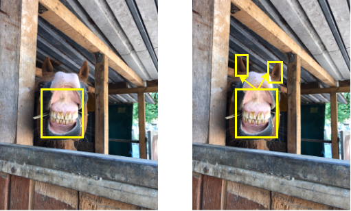
Fig. 81 Attention in visual recognition: In this example attention is first focused on the mouth. With this first perception alone the object can not be recognized. Then attention is focused on something around the mouth. After seeing the ears the object can be recognized to be a horse.

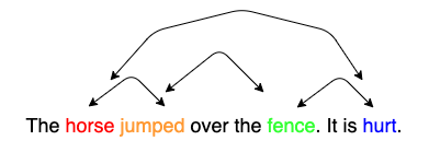
Fig. 82 Attention in reading: When we read horse, we expect to encounter a verb, which is associated to horse. When we read jumped, we expect to encounter a word, which is associated to horse and jumped. When we read hurt, we expect to encounter a word, which is associated to jumped and hurt.

Attention in Neural Networks

In Neural Networks the concept of attention has been introduced in [BCB15]. The main goal was to solve the drawback of Recurrent Neural Networks (RNNs), to be weak in learning long-term-dependencies in sequences. Even though LSTMs or GRUs are better than Vanilla RNNs in this point, they still suffer from the fact that the calculated hidden-state (the compact sequence representation) contains more information from the last few inputs, than from inputs from far behind.

In attention layers the hidden states of all time-steps have an equal chance to contribute to the representation of the entire sequence. The relevance of the individual elements for the entire sequence-representation is learned.

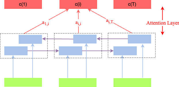
Fig. 83 Attention layer on top of a unidirectional (top) and unidirectional (bottom) RNN, respectively. For each time-step a context vector \(c(i)\) is calculated as a linear combination of all inputs over the entire sequence.

As sketched in the image above, in an attention layer, for each time-step a context vector \(c(i)\) is calculated as a linear combination of all inputs over the entire sequence. The coefficients of the linear combination, \(a_{i,j}\) are learned from training data. In contrast to usual weights \(w_{i,j}\) in a neural network, these coefficients vary with the current input. A high value of \(a_{i,j}\) means that for calculating the \(i.th\) context vector \(c(i)\), in the current input the \(j.th\) element is important - or attention is focused on the j.th input.

An Attention layer can be integrated into a Seq2Seq-Encoder-Decoder architecture as sketched in the image below. Of course, there are many other ways to embed attention layers in Neural Networks, but here we first focus on the sketched architecture.

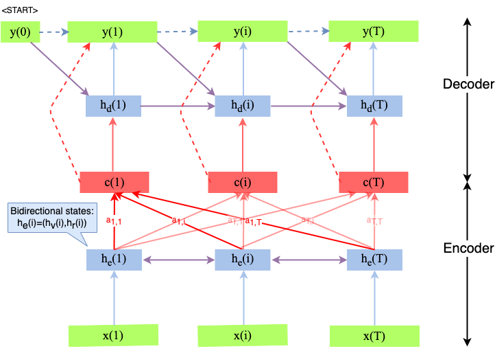
Fig. 84 Attention layer in an Seq2Seq-Encoder-Decoder, applicable e.g. for language modelling or machine translation.

In an architecture like depicted above, the Decoder is trained to predict the probability-distribution for the next word \(y_i\), given the context vector \(c_i\) and all the previously predicted words \(\lbrace y_1,\ldots,y_{i-1}\rbrace\):

\[ p(y_i|\lbrace y_1,\ldots,y_{i-1}\rbrace,c) = g(y_{i-1},h_{d,i},c_i), \]

with

\[ h_{d,i} = k(y_{i-1},h_{d,i-1},c_i) \quad \forall i \in [1,T], \]

The context vector \(c_i\) is

\[ c_{i}=\sum\limits_{j=1}^{T_x} a_{i,j}h_{e,j}, \]

where the concatenated hidden state of the bi-directional LSTM is

\[ h_{e,j}=(h_{v,j},h_{r,j}). \]

The learned coefficients \(a_{i,j}\) describe how well the two tokens (words) \(x_j\) and \(y_i\) are aligned.

\[ a_{i,j} = \frac{\exp(e_{i,j})}{\sum_{k=1}^{T_x}\exp(e_{i,k})}, \]

where

\[ e_{i,j}=a(h_{d,i-1},h_{e,j}) \]

is an alignment model, which scores how well the inputs around position \(j\) and the output at position \(i\) match.

The scoring function \(a()\) can be realized in different ways 1. E.g. it can just be the scalar product

\[ e_{i,j}=h_{d,i-1}^T*h_{e,j}. \]

Another approach is to implement the scoring function as a MLP, which is jointly trained with all other parameters of the network. This approach is depicted in the image below. Note that the image refers to an architecture, where the Attention layer is embedded into a simple Feed-Forward Neural Network. However, this type of scoring can also be applied in the context of a Seq2Seq-Encoder-Decoder architecture. In order to calculate coefficient \(a_j\), the j.th input \(h_j\) is passed to the input of the MLP. The output \(e_j\) is then passed to a softmax activation function:

\[ a_{j} = \frac{\exp(e_{j})}{\sum_{k=1}^{T_x}\exp(e_{k})}%, \quad e_{j}=a(h_{e,j}) \]

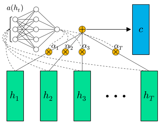
Fig. 85 Scoring function \(a()\) realized by a MLP with softmax-activation at the output. Here, the attention layer is not embedded in as Seq2Seq Encoder-Decoder architecture, but in a Feed-Forward Neural Network. Image Source: [RE16].

Transformer

Motivation

Deep Learning needs huge amounts of training data and correspondingly high processing effort for training. In order to cope with this processing complexity, GPUs/TPUs must be applied. However, GPUs and TPUs yield higher training speed, if operations can be parallelized. The drawback of RNNs (of any type) is that the recurrent connections can not be parallelized. Transformers [VSP+17] exploit only Self-Attention, without recurrent connections. So they can be trained efficiently on GPUs. In this section first the concept of Self-Attention is described. Then Transformer architectures are presented.

Self Attention

As described above, in the Attention Layer }

\[ e_{i,j}=a(h_{d,i-1},h_{e,j}) \]

is an alignment model, which scores how well the input-sequence around position \(j\) and the output-sequence at position \(i\) match. Now in Self-Attention

\[ e_{i,j}=a(h_{i},h_{j}) \]

scores the match of different positions \(j\) and \(i\) of the sequence at the input. In the image below the calculation of the outputs \(y_i\) in a Self-Attention layer is depicted. Here,

• \(x_i * x_j\) is the scalar product of the two vectors.

• \(x_i\) and \(x_j\) are learned such, that their scalar product yields a high value, if the output strongly depends on their correlation.

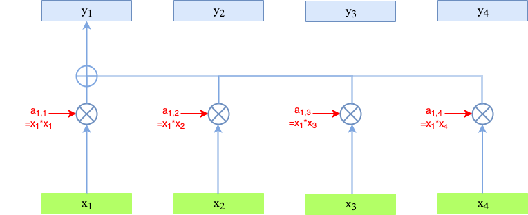
Fig. 86 Calculation of \(y_1\).

Fig. 87 Calculation of Self-Attention outputs \(y_1\) (top) and \(y_2\) (bottom), respectively.

Contextual Embeddings

What is the meaning of the outputs of a Self-Attention layer? To answer this question, we focus on applications, where the inputs to the network \(x_i\) are sequences of words. In this case, words are commonly represented by their embedding vectors (e.g. Word2Vec, Glove, Fasttext, etc.). The drawback of Word Embeddings is that they are context free. E.g. the word tree has an unique word embedding, independent of the context (tree as natural object or tree as a special type of graph). On the other hand, the elements \(y_i\) of the Self-Attention-Layer output \(\mathbf{y}=(y_1,y_2,\ldots y_{T})\) can be considerd to be contextual word embeddings! The representation \(y_i\) is a contextual embedding of the input word \(x_i\) in the given context.

Queries, Keys and Values

As depicted in figure Self-Attention, each input vector \(x_i\) is used in 3 different roles in the Self Attention operation:

• Query: It is compared to every other vector to establish the weights for its own output \(y_i\)

• Key: It is compared to every other vector to establish the weights for the output of the j-th vector \(y_j\)

• Value: It is used as part of the weighted sum to compute each output vector once the weights have been established.

In a Self-Attention Layer, for each of these 3 roles, a separate version of \(x_i\) is learned:

• the Query vector is obtained by multiplying input vector \(x_i\) with the learnable matrix \(W_q\):

\[ q_i=W_q x_i \]

• the Key vector is obtained by multiplying input vector \(x_i\) with the learnable matrix \(W_k\):

\[ k_i=W_k x_i \]

• the Value vector is obtained by multiplying input vector \(x_i\) with the learnable matrix \(W_v\):

\[ v_i=W_v x_i \]

Applying these three representations the outputs \(y_i\) are calculated as follows:

(101)\[\begin{split} a'_{i,j} & = & q_i^T k_j \\ a_{i,j} & = & softmax(a'_{i,j}) \\ y_i & = & \sum_j a_{i,j} v_j \end{split}\]

The image below visualizes this calculation:

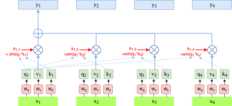
Fig. 88 Calculation of Self-Attention outputs \(y_1\) from queries, keys and values of the input-sequence

In the calculation, defined in (101), the problem is that the softmax-function is sensitive to large input values in the sense that for large inputs most of the softmax outputs are close to 0 and the corresponding gradients are also very small. The effect is very slow learning adaptations. In order to circumvent this, the inputs to the softmax are normalized:

\[\begin{split} a'_{i,j} & = & \frac{q_i^T k_j}{\sqrt{d}} \\ a_{i,j} & = & softmax(a'_{i,j}) \end{split}\]

Multi-Head Attention and Positional Encoding

There are 2 drawbacks of the approach as introduced so far:

1. Input-tokens are processed as unordered set, i.e. order-information is ignored. For example the output \(y_{passed}\) for the input Bob passed the ball to Tim would be the same as the output \(y_{passed}\) for the input Tim passed the ball to Bob.

2. For a given pair of input-tokens \(x_i, x_j\) query \(q\) and key \(k\) are always the same. Therefore their attention coefficien \(a_{ij}\) is also always the same. However, the correlation between a given pair of tokens may vary. In some contexts their interdependence may be strong, in others weak.

These problems can be circumvented by Multi-Head-Attention and Positional Encoding.

Multi-Headed Self-Attention provides an additional degree of freedom in the sense, that multiple (query,key,value) triples for each pair of positions \((i,j)\) can be learned. For each position \(i\), multiple \(y_i\) are calculated, by applying the attention mechanism, as introduced above, \(h\) times in parallel. Each of the \(h\) elements is called an attention head. Each attention head applies its own matrices \(W_q^r, W_k^r, W_v^r\) for calculating individual queries \(q^r\), keys \(k^r\) and values \(v^r\), which are combined to the output:

\[ \mathbf{y}^r=(y^r_1,y^r_2,\ldots y^r_{T_y}). \]

The length of the input vectors \(x_i\) is typically \(d=256\). A typical number of heads is \(h=8\). For combining outputs of the \(h\) heads to the overall output-vector \(\mathbf{y}^r\), there exists 2 different options:

• Option 1:

  • Cut vectors \(x_i\) in \(h\) parts, each of size \(d_s\)

  • Each of these parts is fed to one head

  • Concatenation of \(y_i^1,\ldots,y_i^h\) yields \(y_i\) of size \(d\)

  • Multiply this concatenation with matrix \(W_O\), which is typically of size \(d \times d\)

• Option 2:

  • Fed entire vector \(x_i\) to each head.

  • Matrices \(W_q^r, W_k^r,W_v^r\) are each of size \(d \times d\)

  • Concatenation of \(y_i^1,\ldots,y_i^h\) yields \(y_i\) of size \(d \cdot h\)

  • Multiply this concatenation with matrix \(W_O\), which is typically of size \(d \times (d \cdot h)\)

Fig. 89 Single-Head Self-Attention: Calculation of first element \(y_1\) in output sequence.

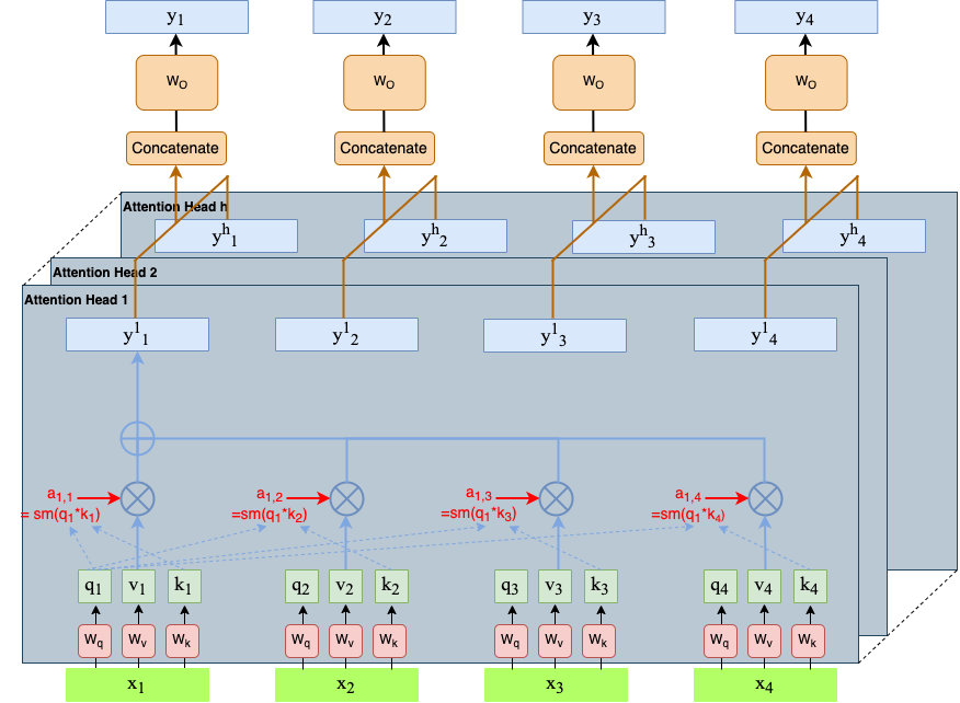
Fig. 90 Multi-Head Self-Attention: Combination of the individual heads to the overall output.

Positional Encoding: In order to embed information to distinguish different locations of a word within a sequence, a positonal-encoding-vector is added to the word-embedding vector \(x_i\). Certainly, each position \(i\) has it’s own positional encoding vector.

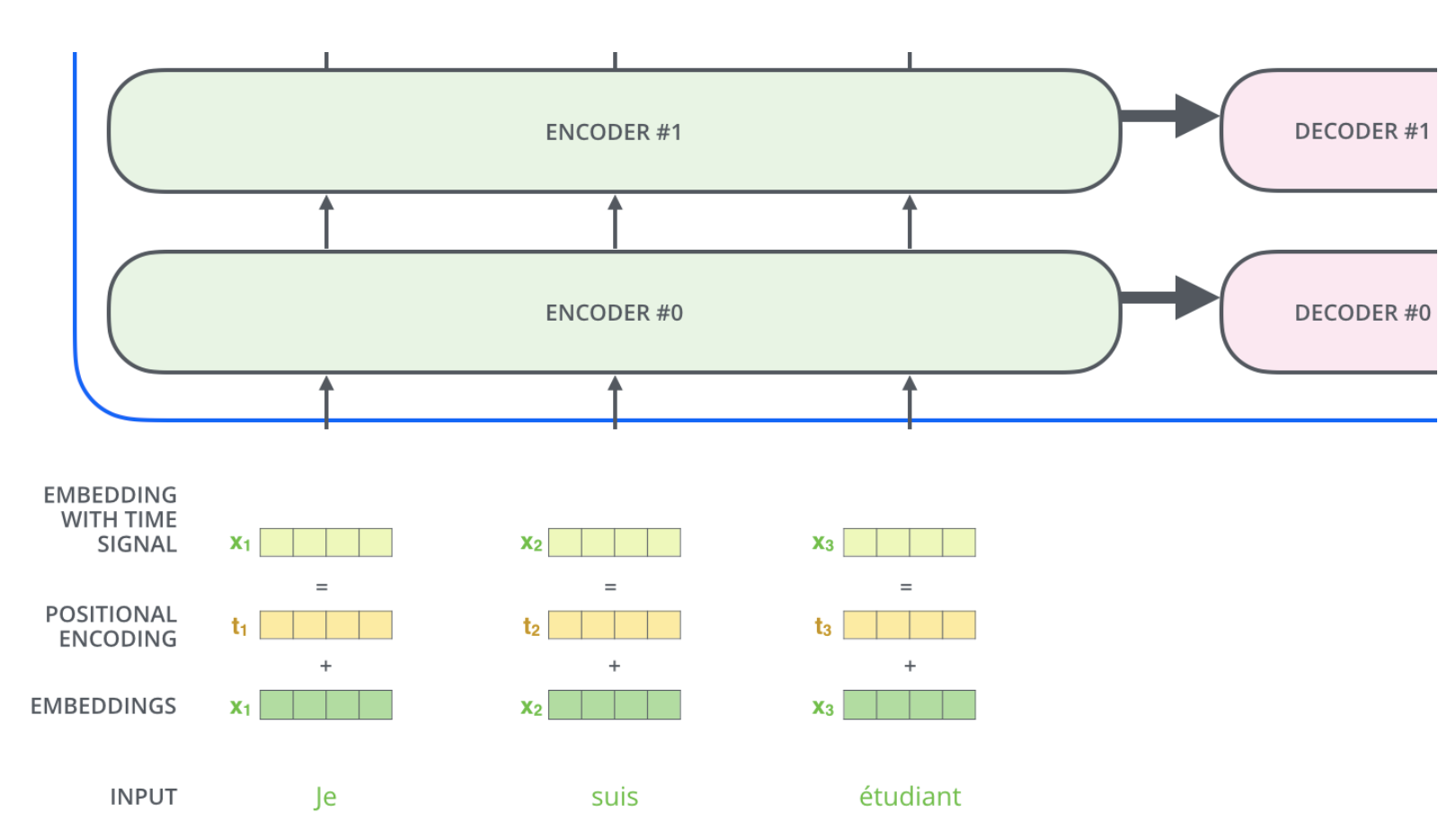
Fig. 91 Add location-specific positional encoding vector to word-embedding vector \(x_i\). Image source: http://jalammar.github.io/illustrated-transformer

The vectors for positional encoding are designed such that the similiarity of two vectors decreases with increasing distance between the positions of the tokens to which they are added. This is illustrated in the image below:

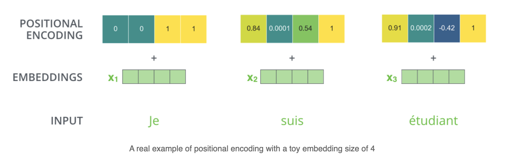
Fig. 92 Positional Encoding: To each position within the sequence a unique positional-encoding-vector is assigned. As can be seen the euclidean distance between vectors for further away positions is larger than the distance between vectors, which belong to positions close to each other. http://jalammar.github.io/illustrated-transformer

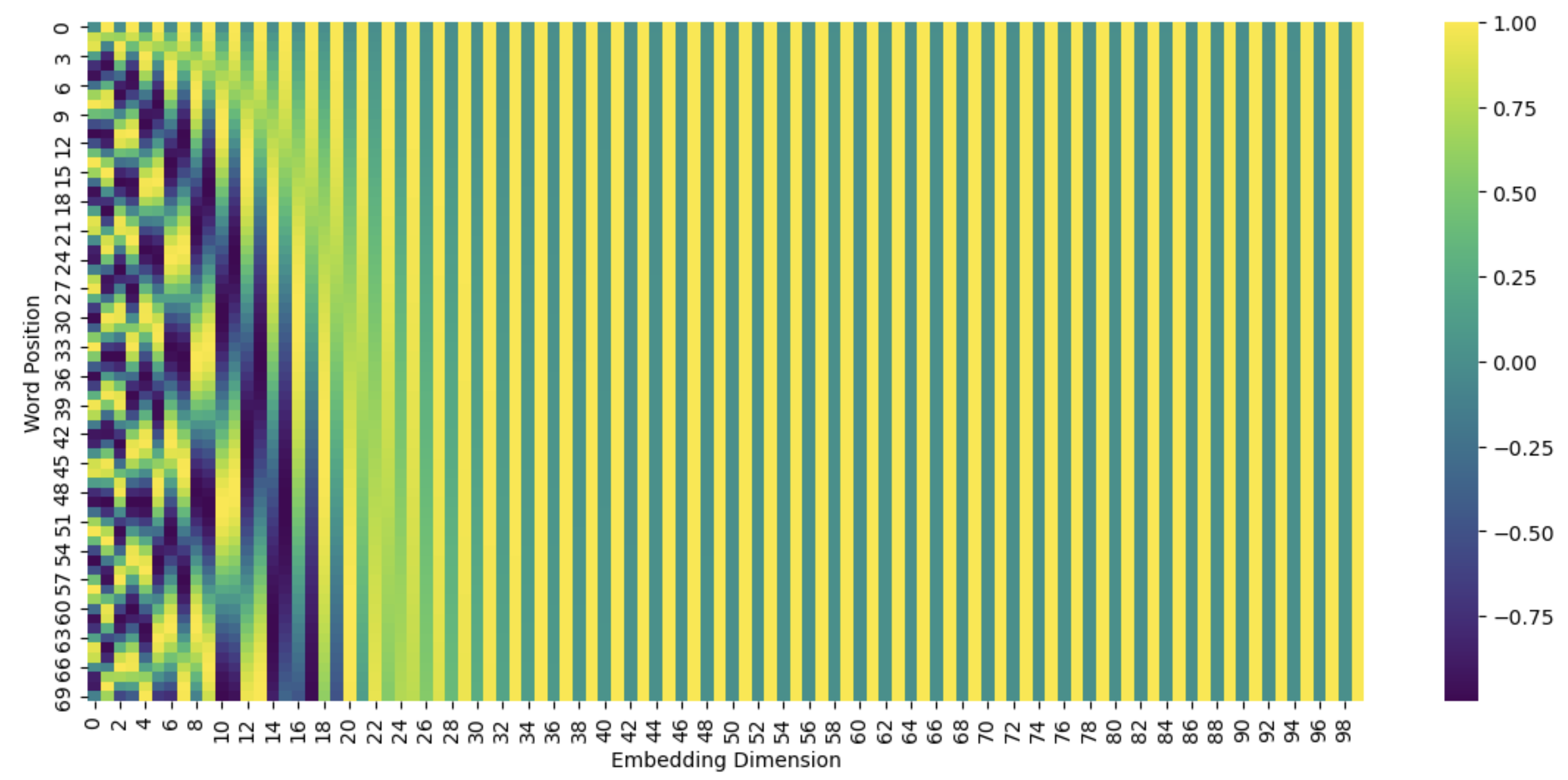
Fig. 93 Visualisation of true positional encoding in BERT

Example

For the two-word example sentence Thinking Machines and for the case of a single head, the calculations done in the Self-Attention block, as specified in Image Singlehead Self-attention, are sketched in the image below. In this example postional encoding has been omitted for sake of simplicity.

Fig. 94 Example: Singlehead Self-Attention for the two-words sequence Thinking Machines . Image source: http://jalammar.github.io/illustrated-transformer

Instead of calculating the outputs \(z_i\) of a single head individually all of them can be calculated simultanously by matrix multiplication:

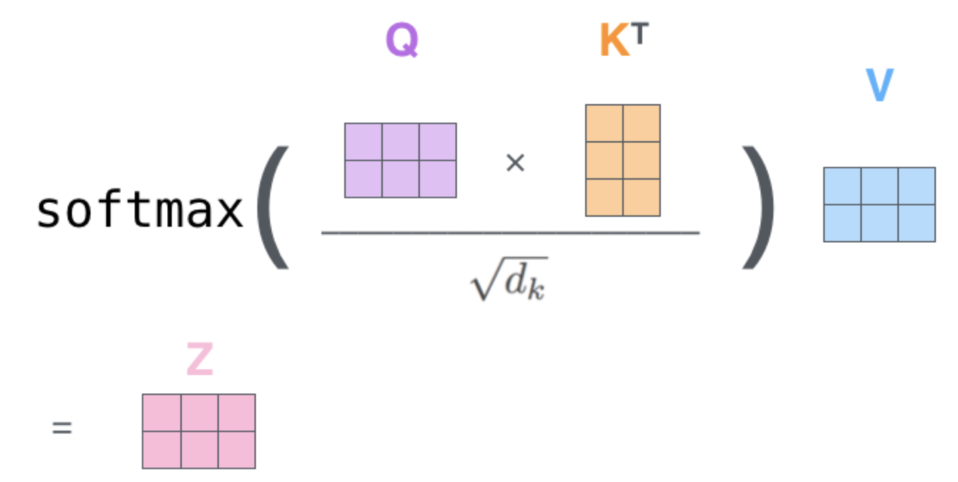
Fig. 95 Calculating all Self-Attention outputs \(z_i\) by matrix-multiplication (Single head). Image source: http://jalammar.github.io/illustrated-transformer

And for Multi-Head Self-Attention the overall calculation is as follows:

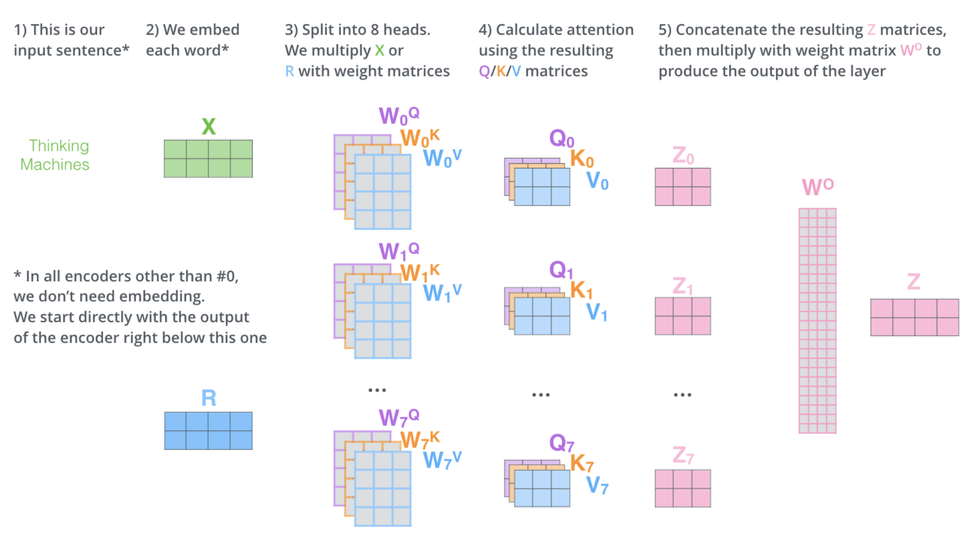
Fig. 96 Calculating all Self-Attention outputs \(z_i\) by matrix-multiplication (Single head). Image source: http://jalammar.github.io/illustrated-transformer

Building Transformers from Self-Attention-Layers

As depicted in the image below, a Transformer in general consists of an Encoder and a Decoder stack. The Encoder is a stack of Encoder-blocks. The Decoder is a stack of Decoder-blocks. Both, Encoder- and Decoder-blocks are Transformer blocks. In general a Transformer Block is defined to be any architecture, designed to process a connected set of units - such as the tokens in a sequence or the pixels in an image - where the only interaction between units is through self-attention.

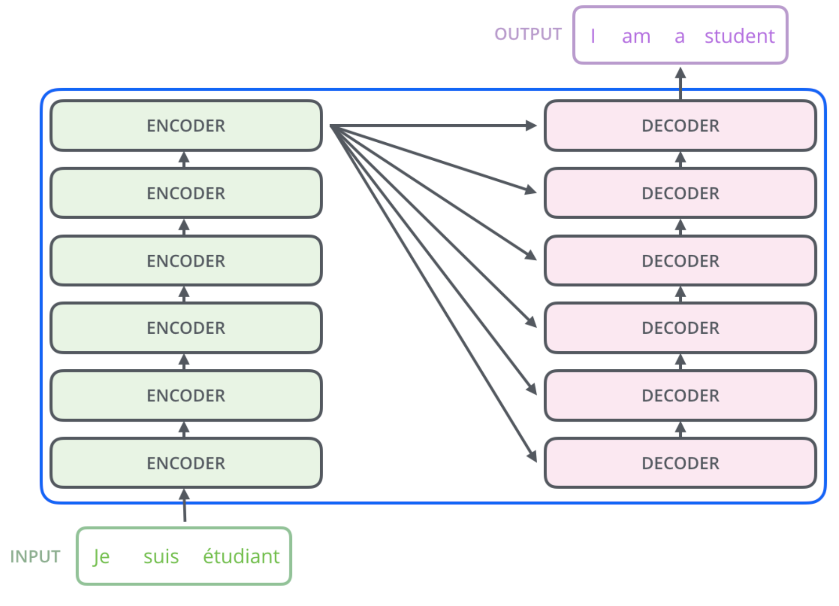
Fig. 97 Encoder- and Decoder-Stack of a Transformer. Image source: http://jalammar.github.io/illustrated-transformer

A typical Encoder block is depicted in the image below. In this image the Self-Attention module is the same as already depicted in Image Multihead Self-attention. The outputs \(z_i\) of the Self-Attention module are exactly the contextual embeddings, which have been denoted by \(y_i\) in Image Multihead Self-attention. Each of the outputs \(z_i\) is passed to a Multi-Layer Perceptron (MLP). The outputs of the MLP are the new representations \(r_i\) (one for each input token). These outputs \(r_i\) constitute the inputs \(x_i\) to the next Encoder block.

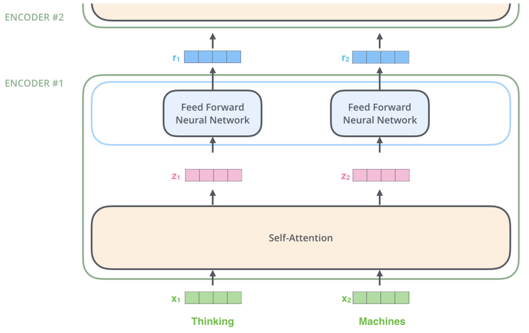
Fig. 98 Encoder Block - simple variant: Self-Attention Layer followed by Feed Forward Network. Image source: http://jalammar.github.io/illustrated-transformer

The image above depicts a simple variant of an Encoder block, consisting only of Self-Attention and a Feed Forward Neural Network. A more complex and more practical option is shown in the image below. Here, short-cut connections from the Encoder-block input to the output of the Self-Attention Layer are implemented. The concept of such short-cuts has been introduced and analysed in the context of Resnet ([HZRS15]). Moreover, the sum of the Encoder-block input and the output of the Self-Attention Layer is layer-normalized (see [BKH16]), before it is passed to the Feed Forward Net.

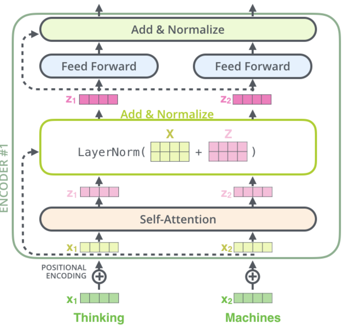
Fig. 99 Encoder Block - practical variant: Short-Cut Connections and Layer Normalisation are applied in addition to Self-Attention and Feed Forward Network. Image source: http://jalammar.github.io/illustrated-transformer

Image Encoder-Decoder illustrates the modules of the Decoder block and the linking of Encoder and Decoder. As can be seen a Decoder block integrates two types of attention:

• Self-Attention in the Decoder: Like the Encoder block, this layer calculates queries, keys and values from the output of the previous layer. However, since Self Attention in the Decoder is only allowed to attend to earlier positions2 in the output sequence future tokens (words) are masked out.

• Encoder-Decoder-Attention: Keys and values come from the output of the Encoder stack. Queries come from the output of the previous layer. In this way an alignment between the input- and the output-sequence is modelled.

On the top of all decoder modules a Dense Layer with softmax-activation is applied to calculate the most probable next word. This predicted word is attached to the decoder input sequence for calculating the most probable word in the next time step, which is then again attached to the input in the next time-step …

In the alternative Beam Search not only the most probable word in each time step is predicted, but the most probable B words can be predicted and applied in the input of next time-step. The parameter \(B\) is called Beamsize.

Fig. 100 Encoder- and Decoder Stack in a Transformer http://jalammar.github.io/illustrated-transformer

In the image below the iterative prediction of the tokens of the target-sequence is illustrated. In iteration \(i=4\) the \(4.th\) target token must be predicted. For this the decoder takes as input the \(i-1=3\) previous estimations and the keys and the values from the Encoder stack.

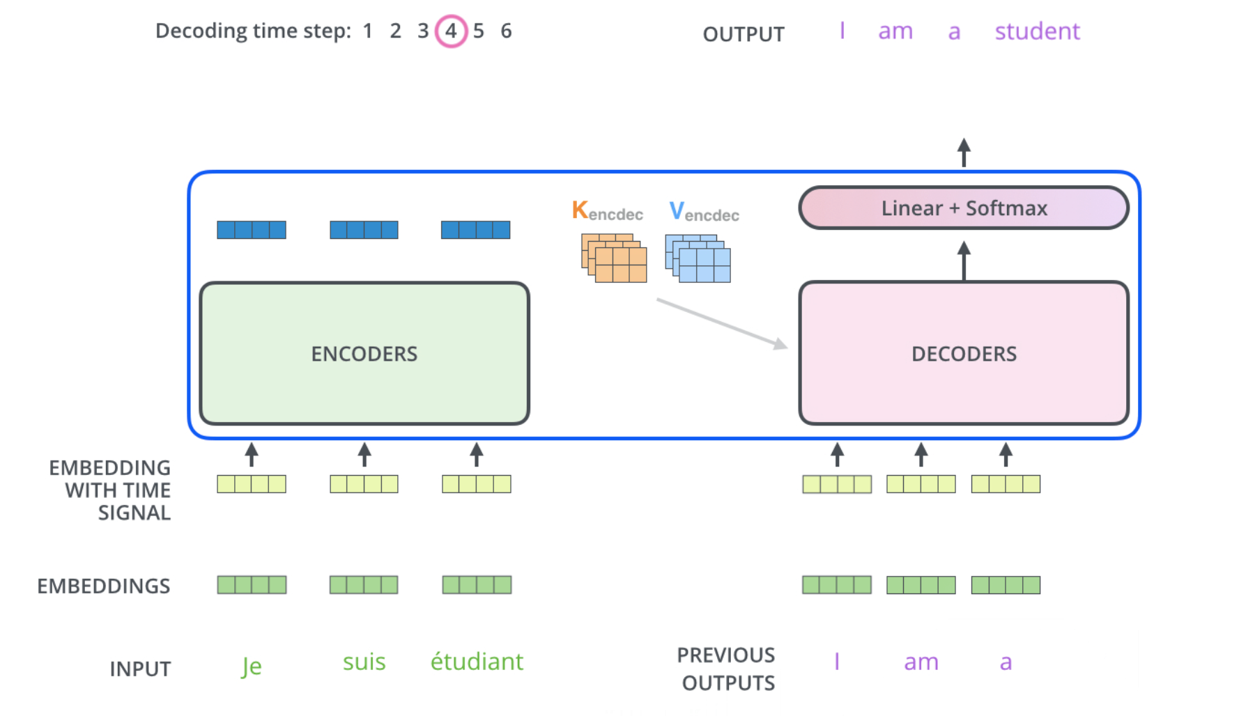
Fig. 101 Prediction of the 4.th target word, given the 3 previously predictions . Image source: http://jalammar.github.io/illustrated-transformer

BERT

BERT (Bidirectional Encoder Representations from Transformers) has been introduced in [DCLT19]. BERT is a Transformer. As described above, Transformers often contain an Encoder- and a Decoder-Stack. However, since BERT primarily constitutes a Language Model (LM), it only consists of an Encoder. When it was published in 2019, BERT achieved state-of-the-art or even better performance in 11 NLP tasks, including the GLUE benchmark3. Pre-trained BERT models can be downloaded, e.g. from Google’s Github repo, and easily be adapted and fine-tuned for custom NLP tasks.

BERT’s main innovation is that it defines a Transformer, which bi-directionally learns a Language Model. As sketched in image Comparison with GPT-1 and Elmo, previous Deep Neural Network LM, where either

• Forward Autoregressive LM: predicts for a given sequence \(x_1,x_2,... x_k\) of \(k\) words the following word \(x_{k+1}\). Then it predicts from \(x_2,x_3,... x_{k+1}\) the next word \(x_{k+2}\), and so on, or

• Backward Autoregressive LM: predicts for a given sequence \(x_{i+1}, x_{i+2},... x_{i+k}\) of \(k\) words the previous word \(x_{i}\). Then it predicts from \(x_{i}, x_{i+1},... x_{i+k-1}\) the previous word \(x_{i-1}\), and so on.

BERT learns bi-directional relations in text, by a training approach, which is known from Denoising Autoencoders: The input to the network is corrupted (in BERT tokens are masked out) and the network is trained such that its output is the original (non-corrupted) input.

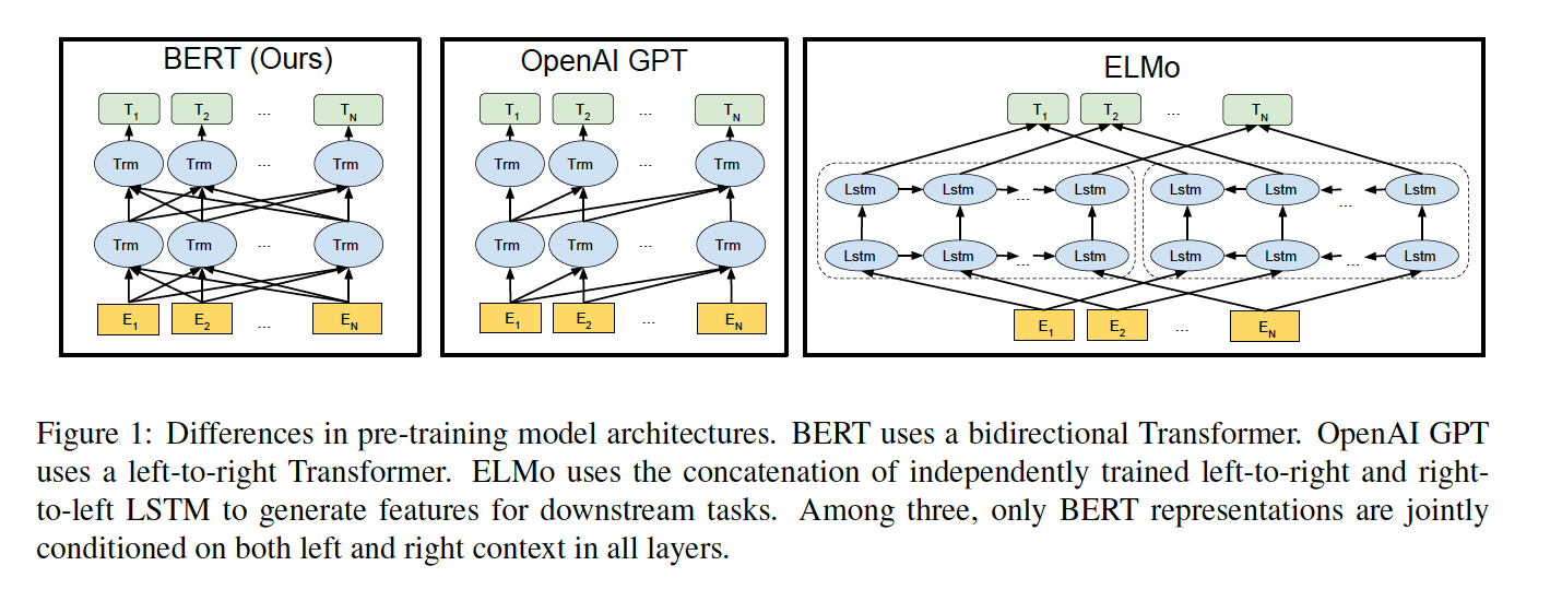
Fig. 102 Prediction of the 4.th target word, given the 3 previously predictions. Image source: [DCLT19]

BERT training is separated into 2 stages: Pre-Training and Fine-Tuning. During Pre-Training, the model is trained on unlabeled data for the tasks Masked Language Model (MLM) and Next Sentence Prediction (NSP). Fine-Tuning starts with the parameters, that have been learned in Pre-Training. There exists different downstream tasks such as Question-Answering, Named-Entity-Recognition or Multi Natural Language Inference, for which BERT’s parameters can be fine-tuned. Depending on the Downstream task, the BERT architecutre must be slightly adapted for Fine-Tuning.

Fig. 103 BERT: Pretraining on tasks Masked Language Model and Next Sentence Prediction, followed by task-specific Fine-Tuning. Image source: [DCLT19]

In BERT, tokens are not words, but word-pieces. This yields a better out-of-vocabulary-robustness.

BERT Pre-Training

Masked Language Model (MLM): For this \(15\%\) of the input tokens are masked at randomly. Since the \([ MASK ]\) token is not known in finetuning not all masked tokens are replaced by this marker. Instead

• \(80\%\) of the masked tokens are replaced by \([ MASK ]\)

• \(10 \%\) of them are replaced by a random other token.

• \(10 \%\) of them remain unchanged.

These masked tokens are predicted by passing the final hidden vectors, which belong to the masked tokens to an output softmax over the vocabulary. The Loss function, which is minimized during training, regards only the prediction of the masked values and ignores the predictions of the non-masked words. As a consequence, the model converges slower than directional models, but has increased context awareness.

Next Sentence Prediction (NSP):

For NSP pairs of sentences \((A,B)\) are composed. For about \(50\%\) of these pairs the second sentence \(B\) is a true successive sentence of \(A\). In the remaining \(50\%\) \(B\) is a randomly selected sentence, independent of sentence \(A\). The BERT architecture is trained to estimate if the second sentence at the input is a true successor of \(A\) or not. The pairs of sentences at the input of the BERT-Encoder stack are configured as follows:

• A \([CLS]\) token is inserted at the beginning of the first sentence and a \([SEP]\) token is inserted at the end of each sentence.

• A sentence embedding indicating Sentence \(A\) or Sentence \(B\) is added to each token. These sentence embeddings are similar in concept to token embeddings with a vocabulary of 2.

• A positional embedding is added to each token to indicate its position in the sequence.

Fig. 104 Input of sentence pairs to BERT Encoder stack. Segment Embedding is applied to indicate first or second sentence. Image source: [DCLT19]

For the NSP task a classifier is trained, which distinguishes successive sentences and non-successive sentences. For this the output of the \([CLS]\) token is passed to a binary classification layer. The purpose of adding such Pre-Training is that many NLP tasks such as Question-Answering (QA) and Natural Language Inference (NLI) need to understand relationships between sentences.

BERT Fine-Tuning

For each downstream NLP task, task-specific inputs and outputs are applied to fine-tune all parameters end-to-end. For this minor task-specific adaptations at the input- and output of the architecture are required.

• Classification tasks such as sentiment analysis are done similarly to NSP, by adding a classification layer on top of the Transformer output for the [CLS] token.

• In Question Answering tasks (e.g. SQuAD v1.1), the software receives a question regarding a text sequence and is required to mark the answer in the sequence. The model can be trained by learning two extra vectors that mark the beginning and the end of the answer.

• In Named Entity Recognition (NER), the software receives a text sequence and is required to mark the various types of entities (Person, Organization, Date, etc) that appear in the text. The model can be trained by feeding the output vector of each token into a classification layer that predicts the NER label.

Fig. 105 BERT Fine-Tuning. Image source: [DCLT19]

Contextual Embeddings from BERT

Instead of fine-tuning, the pretrained token representations from any level of the BERT-Stack can be applied as contextual word embedding in any NLP task. Which representation is best depends on the concrete task.

Fig. 106 Contextual Embeddings from BERT. Image source: [DCLT19]

GPT, GPT-2 and GPT-3

In contrast to BERT, which is an encoder-only transformer, GPT ([RN18]), GPT-2 ([RWC+19]) and GPT-3 ([BMR+20]) are decoder-only transformers. Since there is no encoder, there is also no encoder-decoder attention block in the decoder.

The GPT variants are Autoregressive Language Models (AR LM). A AR LM predicts for a given token-sequence \((x_1, x_2, \ldots x_k)\) the following token \(x_{k+1}\). Then it predicts from \((x_2, x_3, \ldots x_{k+1})\) the next word \(x_{k+2}\) and so on. In contrast to BERT it therefore integrates only the previous context. However, since AR LMs can predict the next tokens from given prompts, they are applicable for tasks like generating text or any type of sequence-to-sequence transformations such as translation, text-to-code, etc.

Moreover, the fact that the AR LM is trained for text-completion, the authors of GPT-2 ([RWC+19]) proposed to implement multi-task-learning at a data-level. What does this mean? Usually multi-task-learning is realized not on a data- but on a architectural level. A typical approach is to have a common network-part, e.g. the first layers, which constitutes the feature-extractor, and on top of this common part two or more task-specific architectures in parallel, e.g. one stack of layers for classification, one stack of layers for Named-Entity-Recognition and so on. Each task-specific part is trained with task-specific labeled data. BERT and the first GPT are examples for this approach. The drawback is, that task-specific fine-tuning still requires quite large amounts of data.

In contrast to this architectural solution for multi-task learning, in data-level multi-task learning only one common architecture is applied and the task-description is part of the input data. Instead of predicting

\[ p(output | input), \]

the task-conditioned probability

\[ p(output | input, task) \]

is predicted, i.e. for one and the same input, different outputs can be generated. This is possible if the model is an AR LM, because the input and the task-description are just sequences of tokens. For example the two different tasks translate english to french and translate english to german, can be implemented by providing training data of type

(translate to french, < english text >, < french text >)

and

(translate to german, < english text >, < german text >).

GPT-2 proposes to take data of this format, and just training the model for a text completion objective should suffice to train the model for all the underlying objectives. Since the unsupervised and supervised objectives are the same, the global minima for the unsupervised objective are the same as the global minima for the supervised objective. Moreover, since the model is not trained specifically for any of the underlying tasks (translation, summarization, question-answering, etc.), it is said to be an example of few-shot-, one-shot- or zero-shot learning. In few-shot learning one just has to explain the task and provide a few examples for this task in the inference phase, i.e. there is no task-specific weight adaptation. The concept of the x-shot approaches is depicted in the image below. The fact that no fine-tuning on downstream tasks is required is a step towards general intelligence.

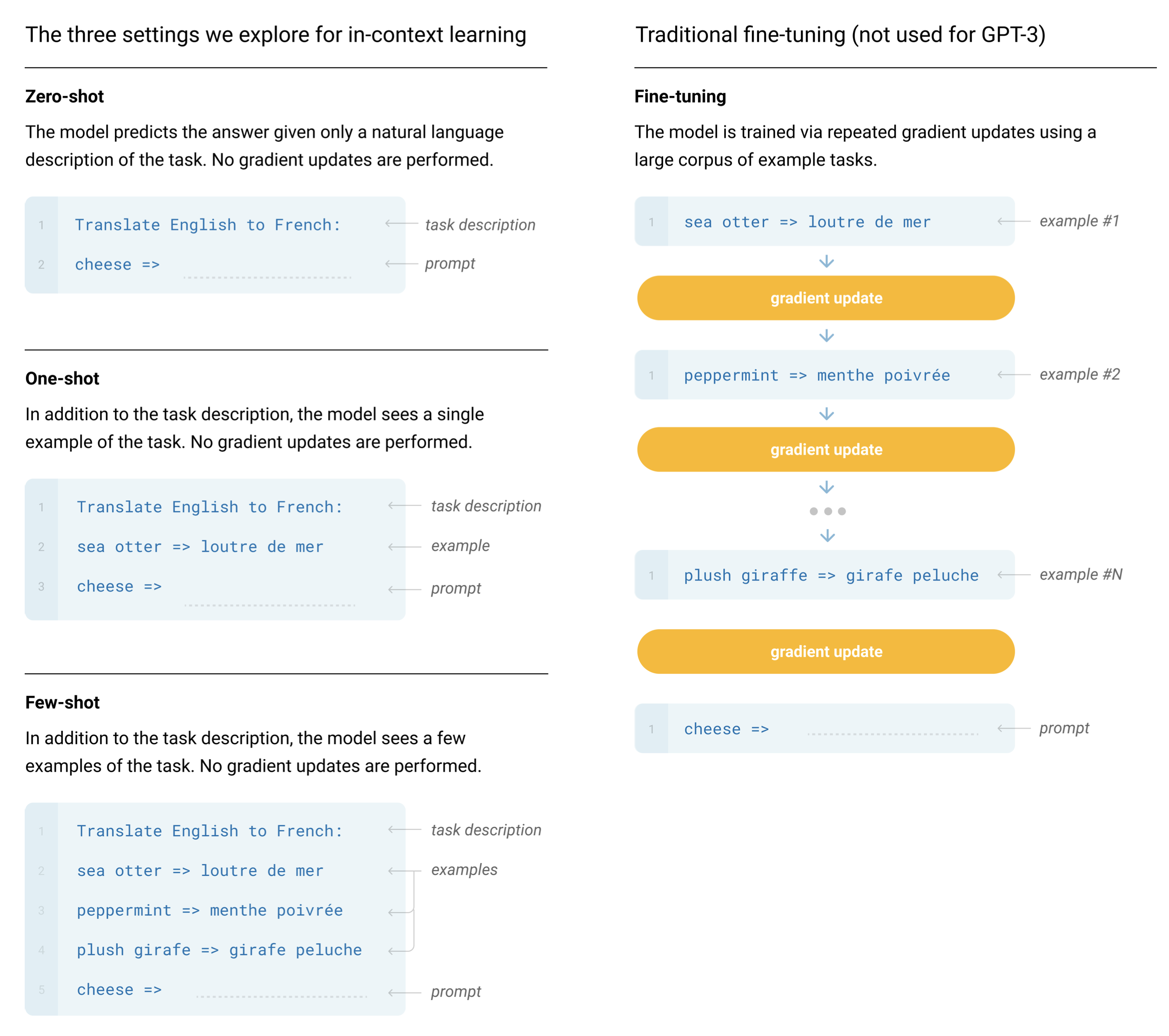
Fig. 107 Image source: [BMR+20]. Zero-shot, one-shot and few-shot, contrasted with traditional fine-tuning. The panels above show four methods for performing a task with a language model. Fine-tuning is the traditional method, whereas zero-, one-, and few-shot, which are applied in GPT-3, require the model to perform the task with only forward passes at test time. In the few shot setting typically a few dozen examples are presented to the model. Exact phrasings for all GPT-3 task descriptions, examples and prompts can be found in Appendix G of the paper.

Of course, before x-shot learning can be applied, the model must be pretrained. GPT is pretrained as a autoregeressive language model from unsupervised data (large amounts of texts).

GPT-3 is evaluated on more than two dozen datasets. For each of these tasks, it is evaluated for 3 settings: zero-shot, one-shot, and few-shot.

The largest GPT-3 model consists of 175 billion parameters, which is 470 times more than BERT, and requires a storage of 800GB. Smaller variants, which have been considered in [BMR+20] are depicted in the table below:

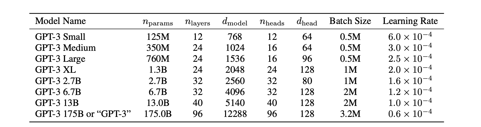
Fig. 108 Image source: [BMR+20]. Sizes, architectures, and learning hyper-parameters (batch size in tokens and learning rate) of the trained models. All models were trained for a total of 300 billion tokens

Summary of main properties:

GPT ([RN18])

• Decoder-only Autoregressive Language Model (AR LM)

• 12 layers decoder with masked self-attention as in decoder of [VSP+17] and 12 heads.

• At the input: Byte Pair Encoding and positional encoding.

• 768-dimensional token-representations

• 117 Million parameters

• Unsupervised Pretraining and task-specific supervised fine-tuning.

• Trained on BooksCorpus Dataset (7000 unpublished books), 5GB

• already remarkable zero-shot performance on different NLP tasks like question-answering, schema resolution, sentiment analysis only due to pre-training of the AR LM.

GPT-2 ([RWC+19])

• Decoder-only Autoregressive Language Model (AR LM)

• much larger model than GPT: 1.5 billion parameters

• 48 layers

• 1600-dimensional token-representations

• Layer normalisation was moved to input of each sub-block and an additional layer normalisation was added after final self-attention block

• Byte Pair Encoded Input Tokens

• Task-conditioned training (unsupervised)

• Performs well in Zero-Shot-Setting for some NLP tasks

• much larger dataset for training. WebText Corpus (40GB): Scrapped data from Reddit and outbound links

• GPT-2 showed that training on larger dataset and having more parameters improved the capability of language model to understand tasks and surpass the state-of-the-art of many tasks in zero shot settings.

GPT-3 ([BMR+20])

• Decoder-only Autoregressive Language Model (AR LM)

• much larger model than GPT-2: 175 billion parameters

• 96 layers, each having 96 heads

• 12888-dimensional token-representations

• Byte Pair Encoded Input Tokens

• Sparse Attention patterns in Self-Attention blocks

• Task-conditioned training (unsupervised)

• Performs well on Zero-Shot-, One-Shot-, and Few-Shot-settings in downstream NLP tasks.

• Perform well on on-the-fly tasks on which it was never explicitly trained on, like summing up numbers, writing SQL queries and codes

• trained on a mix of five different corpora, each having certain weight assigned to it. High quality datasets were sampled more often, and model was trained for more than one epoch on them. The five datasets used were Common Crawl, WebText2, Books1, Books2 and Wikipedia, 600GB in total.

---

1

An overview for other scoring functions is provided here.

2

The reason for this is that the Decoder caluclates its output (e.g. the translated sentence) iteratievely. In iteration \(i\) the \(i.th\) output of the current sequence (e.g. the i.th translated word) is estimated. The already estimated tokens at positions \(1,2,\ldots, i-1\) are applied as inputs to the Decoder stack in iteration \(i\), i.e. future tokens at positions \(i+1, \ldots\) are not known at this time.

3

GLUE Benchmark for NLP tasks