
Deep Reinforcement Learning
Contents
Deep Reinforcement Learning#
In the previous section Reinforcementlearning has been introduced. For solving the control problem with TD-Learning, Sarsa and Q-Learning has been described. These algorithms estimate \(Q(S,A)\) -values for each possible state-action pair \((S,A)\). From the estimated \(Q(S,A)\)-values the policy can easily be derived by selecting in each state \(S\) the action \(A\), which has the maximum \(Q(S,A)\)-value in this state. In order to estimate the \(Q(S,A)\) reliably, each state-action pair must be traversed multiple times. This is not feasible for many real-world problems, where the number of possible state-actions pair is very large. For example, in Backgammon alone the number of states is estimated to be in the range of \(10^{20}\) and the number of state-action pairs is correspondingly higher.
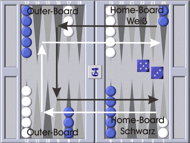
Fig. 72 In Backgammon alone the number of states is estimated to be in the range of \(10^{20}.\)#
The problem, that a multiple traversion of all state action pairs is not feasible, is solved by learning a regression model, i.e. a function, which maps Q-Values to each possible state-action pair. In this approach Reinforcement-Learning and Supervised Learning are combined in the way that e.g. Q-Learning is applied to provide \(Q(S,A)\)-values for a limited set of state-action pairs. Then a supervised ML-algorithm, e.g. a MLP, is applied to learn a function
Deep Q-Network (DQN)#
Before the invention of Deep Q-Network (DQN) in [MKS+13], either linear regression models or non-linear conventional neural networks (MLPs) have been applied for learning a good approximation. Training linear models turned out to be stabel, in the sense of convergence. However, they often lacked sufficient accuracy. On the other hand non-linear models turned out to have weak convergence behaviour. This is because ML-algorithms usually assume i.i.d (independent and identical distributed data). However, data provided by the reinforcement-algorithm is sequentially strongly correlated. Moreover, the distribution of data may change abruptly, because a relatively small adaption of the \(Q(S,A)\)-values may yield a totally different policy.
The publication Human-level control through deep reinforcement learning ([MKS+13]) constituted a breakthrough in the combination of Reinforcement Learning and Deep Neural Networks. For some retro Atari computer games such as Pong, Breakout, Seaquest or Space Invaders , the authors managed to learn a good non-linear \(Q(S,A)\)-function with a Convolutional Neural Network (CNN).
In their experiments, the authors applied their DQN to a range of Atari 2600 games implemented in the Arcade Learning Environment1. Atari 2600 is a challenging RL testbed that presents agents with a high dimensional visual input: \(210 \times 160\) RGB video at 60Hz. The only information provided to the DQN has been the screencasts of the computer games.
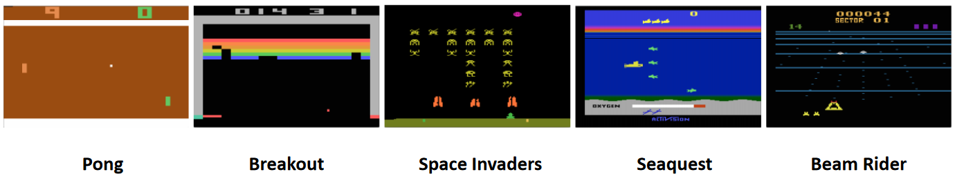
Fig. 73 Screenshots of some classical Atari computer games, for which DQN has been applied to learn a good \(Q(S,A)\)-function.#
In this subsection the concept of DQN, as developed in [MKS+13], will be described.
DQN Architecture and Preprocessing#
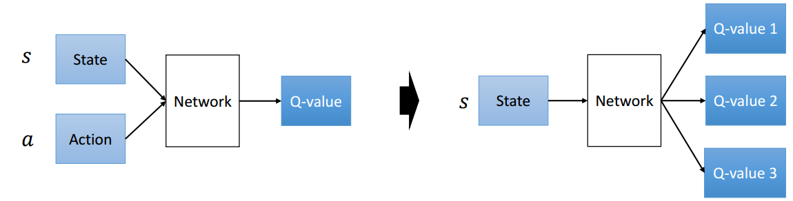
Fig. 74 Predicting a Q-value for each state-action pair at the input of a network is conceptionally the same as predicting for a given input state a Q-value for each possible action. Image Source: http://ir.hit.edu.cn/~jguo/docs/notes/dqn-atari.pdf#
The input to the CNN represents the current game state. The output of the DQN has as much elements as the maximal number of actions available. Atari classical games have been controlled by a joystick, which provides 18 different postions. For each of these 18 actions one Q-value is estimated for the current input state.

The input to the network represents the current game state. In general a state should always contain as much as relevant information as possible. In computer games movement is obviously a relevant information. Since movement can not be obtained by observing only a single frame of the screencast, four successive frames are applied to the input of the network. However, these frames are not directly passed to the first layer of the CNN, instead a preprocessed version of 4 successive frames of the screencast are used.
The preprocessing function takes \(m=4\) successive RGB-frames of size \(210 \times 160\) from the Atari 2600 emulator. Next, for any pair of 2 successive frames at each pixel-position the maximum value within this pair of frames is determined. The smaller value is ignored in the sequel. This maximum-operation is necessary, because in the videos some objects are represented only in the even frames, others only in the odd frames. The RGB-frames are then transformed to YCrCb and only the luminance channel Y is regarded in the sequel, whereas the two chromatic channels are ignored. The Y-channel frames are then rescaled to a size of \(84 \times 84\). The resulting tensor of size \(84 \times 84 \times 3\) constitutes the input to the first layer of the CNN. The details of the CNN, containing 3 convolutional and 2 fully connected layers, are given in the table below.

Fig. 76 Hyperparameters of the DQN CNN. Image Source: [MKS+13]#
DQN Learning#
As already mentioned above, the idea of the Deep Q-Network in general is to
Apply an emulator, which models the environment. The emulator provides for each state \(s\) the set of possible actions \(A(s)\). Moreover, the emulator allows to select for the given state \(s\) a corresponding action \(a \in A(s)\) and the possibility to execute this action. For action-selection e.g. the \(\epsilon\)-greedy policy an be applied (see previous page). After the execution of \(a\) the emulator returns the obtained reward \(r\) and the new state \(s'\). Starting from an arbitrary initial state one can thus select a set \(D\) of quadruples \((s,a,r,s')\). The quadruple set \(D\) is called Replay Memory.
Apply the quadruple-set \(D\) as training-data for the deep neural network, which learns a function \(f: (S,A) \rightarrow Q(S,A)\).
During training, the weights \(\Theta\) of the DQN are iteratively adapted such that a Loss-Function is minimzed (this learning-approach is called (Stochastic) Gradient Descent). The loss-function in general somehow measures the difference between the current network output and the corresponding target value. For the given DQN the network outputs are \(Q(s,a,\Theta)\)-values for a given quadruple \((s,a,r,s')\) at the input with the current network-weights \(\Theta\). But what are the target values? In Q-learning the state-action-value-update rule, as already defined in equation (100), is
where \(s\) is the current state, \(a\) is the chosen action, \(r\) is the obtained reward, \(s'\) is the obtained successor state, and \(a'\) is a possible action in the successor state \(s'\). In this iterative update-process old values \(Q(s,a)\) are updated by new experiences \(r + \gamma \max\limits_a' Q(s',a')\). These new experiences are applied as target-values. For computing these target values \(r\) and \(s'\) are given from the current quadruple \((s,a,r,s')\), but what about \(\max\limits_a' Q(s',a')\)? The answer is to calculate the \(Q(s',a')\) with the DQN, however not with the current weights \(\Theta\), but with an older version \(\Theta^{-}\). The values of this older version are denoted by \(\hat{Q}(s',a')\). This older version is only applied to calculate the targets. The weights of the older version are updated from time to time. In this way DQN-learning realizes the same concept as the state-action-value-update rule of Q-learning: in both algorithms \(Q(s,a)\) are iteratively updated by the experienced reward \(r\) and the best \(Q(s',a')\)-value in the experienced successor state \(s'\) and both algorithms apply older \(\hat{Q}(s',a')\)-values for this update. In DQN the weights are updated per minibatch, where a minibatch is a random sample from the Replay Memory \(D\).
Deep Q-Learning Algorithm
Initialize Replay Memory \(D\) to capacity \(N\)
Initialize action-value-function \(Q\) with random weights \(\theta\)
Initialize target action-value-function \(\hat{Q}\) with weights \(\theta^{-}=\theta\)
For episode from 1 to M do
Initialize sequence \(s_1=\{x_1\}\) and preprocess sequence \(\phi_1=\phi(s_1)\)
For t from 1 to T do
With probability \(\epsilon\) select a random action \(a_t\), otherwise select \(a_t=argmax_a(Q(\phi(s_t),a;\theta))\)
Execute \(a_t\) in emulator, observe reward \(r_t\) and image \(x_{t+1}\)
Set \(s_{t+1}=s_t,a_t,x_{t+1}\) and preprocess \(\phi_{t+1}=\phi(s_{t+1})\)
Store transitition \((\phi_t,a_t,r_t,\phi_{t+1})\) in \(D\)
Sample random minibatch of transititions \((\phi_j,a_j,r_j,\phi_{j+1})\) from \(D\)
Set
\[\begin{split} y_j=\left\{ \begin{array}{ll} r_j & \mbox{if episode terminates at step } j+1 \\ r_j + \gamma \max_{a'} \hat{Q}(\phi_{j+1},a';\theta^-) & \mbox{ otherwise } \\ \end{array} \right. \end{split}\]Perform a gradient descent step on \(\left(y_j-Q(\phi_j,a_j;\theta) \right)^2\)} w.r.t. \(\theta\)
Every C steps update \(\hat{Q}=Q\)
In the figure below, the score, achieved by DQN w.r.t. human players is shown for classic Atari games. This score has been calculated by
i.e. a score of 100 corresponds to the score achieved by professional human players. An average human player has a score of \(76\%\).
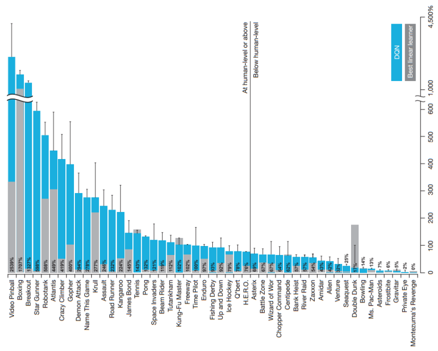
Fig. 77 DQN performance compared to human players. Image Source: [MKS+13]#