Linear Classification#

Simple Linear Classification#

Binary linear Classification by example#

import numpy as np
from matplotlib import pyplot as plt

Given labeled training-data T:

T=np.array([[1,1,0],
         [1,3,0],
         [2,1,0],
         [3,0,0],
         [3,1,1],
         [3,2,1],
         [4,1,1],
         [2,3,1]])

plt.figure(figsize=(10,8))
plt.plot(T[:4,0],T[:4,1],"ob")
plt.plot(T[4:,0],T[4:,1],"xr")
plt.xlabel("$x_1$")
plt.ylabel("$x_2$")
plt.show()

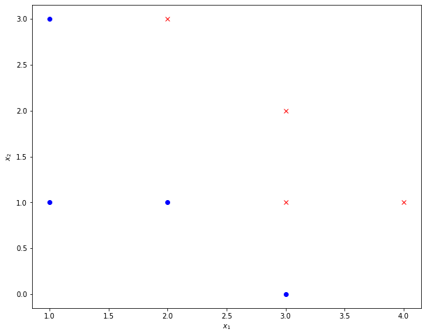
The task is to learn a discrimant

(15)#\[ g(\mathbf{x})=w_0 + w_1 x_1 + w_2 x_2 \]

such that

(16)#\[\begin{split} g(\mathbf{x}) = \left\{ \begin{array}{ll} > 0 & \mbox{ for all }\mathbf{x}_t \mbox{ with } r_t=1 \\ < 0 & \mbox{ for all }\mathbf{x}_t \mbox{ with } r_t=0 \\ \end{array} \right. \end{split}\]

All datapoints \(\mathbf{x}\), which fulfill \(g(\mathbf{x}) = 0\) lie on the discriminator line. I.e.

(17)#\[ g(\mathbf{x})=w_0 + w_1 x_1 + w_2 x_2 =0 \]

is the implicit definiton of the discriminator line.

This implicit line-definition can easily be transformed to the more common line definition of type \(y=mx+b\). Equation (17) is rearranged such that \(x_2\) is isolated:

\[ x_2 = - \frac{w_1}{w_2} x_1 - \frac{w_0}{w_2} \]

In the given example \(x_2\) corresponds to \(y\) and \(x_1\) corresponds to \(x\). Hence the slope of the line is

\[ m = - \frac{w_1}{w_2} \]

and its intersection with the \(x_2\)-axis is:

\[ b= - \frac{w_0}{w_2} \]

A line, which separates the training data, given in this example is:

\[ x_2= 5 - 1.43 x_1 \]

This line is visualized below:

plt.figure(figsize=(10,8))
plt.plot(T[:4,0],T[:4,1],"ob")
plt.plot(T[4:,0],T[4:,1],"xr")
plt.plot([0,3.5],[5,0],"g")
plt.xlabel("$x_1$")
plt.ylabel("$x_2$")
plt.show()

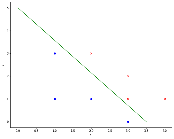
For this line we have a slope of

(18)#\[ \frac{-5}{3.5} = -1.43 = - \frac{w_1}{w_2} \]

and an intersection with the \(x_2\)-axis of

(19)#\[ 5= - \frac{w_0}{w_2} \]

In order to determine the corresponding weights \(w_i\) one can freely choose one arbitrary \(w_i\), e.g. we set

\[ w_2 =1.0 \]

Given this selection we can derive

\[ w_1 = 1.43 \]

from equation (18) and

\[ w_0 = -5 \]

from equation (19).

We can check, if these weights actually fullfill the conditions, given in equation (16) for all elements of the given training data \(T\).

First we evaluate \(g(\mathbf{x})= w_0+w_1 x_1 + w_2 x_2\) for the first 4 training elements, which have a label \(r_t=0\) and we obtain, that for all of them \(g(\mathbf{x})<0\).`

for x in T[:4,:2]:
   print(-5+1.43*x[0]+1*x[1]) 

-2.5700000000000003
-0.5700000000000003
-1.1400000000000001
-0.71

The last 3 training samples have \(r_t=1\), and as shown below for all of them we yield \(g(\mathbf{x})>0\).

for x in T[4:,:2]:
   print(-5+1.43*x[0]+1*x[1]) 

29000000000000004
29
7199999999999998
8599999999999999

Now assume, that we have a new datapoint

\[ x=[2,2.5], \]

which must be classified. For this we just insert this point into \(g(\mathbf{x})\):

output=-5+1.43*2+1*2.5
print(output)

0.3599999999999999

Since we obtain \(g(\mathbf{x})>0\), this datapoint can be assigned to the class with label \(1\).

K-ary linear classification in \(d\)-dimensional space#

In the example above binary linear classification of 2-dimensional input data \(\mathbf{x}\) has been demonstrated. In the general case of \(d\)-dimensional input data, the discriminator equation ((15) for the 2-dimensional case) is:

(20)#\[ g(\mathbf{x})=w_0 + w_1 x_1 + w_2 x_2 + \cdots + w_d x_d \]

The discriminator conditions remain the same as in equation disscond and the equation

(21)#\[ g(\mathbf{x})=w_0 + w_1 x_1 + w_2 x_2 + \cdots + w_d x_d = 0 \]

now defines a \(d-1\) dimensional hyperplane, which discriminates the classes in the \(d\)-dimensional space.

The generalisation from binary classification to \(K\)-ary classification is realized by applying for each of the \(K\) classes one individual equation of type (20):

(22)#\[\begin{split} g_1(\mathbf{x}) = w_{1,0} + w_{1,1} x_1 + w_{1,2} x_2 + \cdots + w_{1,d} x_d \\ g_2(\mathbf{x}) = w_{2,0} + w_{2,1} x_1 + w_{2,2} x_2 + \cdots + w_{2,d} x_d \\ \vdots \\ g_K(\mathbf{x}) = w_{K,0} + w_{K,1} x_1 + w_{K,2} x_2 + \cdots + w_{K,d} x_d \\ \end{split}\]

In this case \(K \cdot (d+1)\) weights \(w_{i,j}\) must be learned. The class labels are \(r_p \in [ 1,2,\ldots K ]\). The weights are learned such that for each training element \((\mathbf{x}_p,r_p)\)

\[ r_p= \mbox{ argmax}_{j} \; g_j(\mathbf{x}_p), \]

i.e. if the current target label is \(r_p=k\), then the output of \(g_k(\mathbf{x}_p)\) must be larger than the output of all other \(K-1\) \(g_i(\mathbf{x}_p)\).

Binary Logistic Regression#

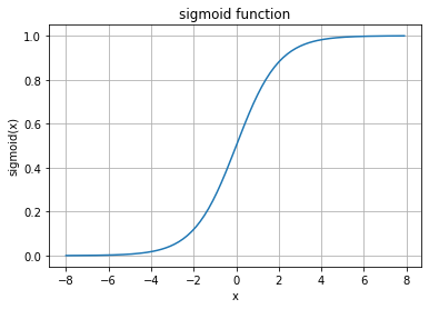
Despite the name Logistic Regression is a binary linear classification as introduced above. The only difference is that in Logistic Regression the output of the discriminator \(g(\mathbf{x})\) is passed to a sigmoid-function. In general, the sigmoid function is defined as follows:

\[ sigmoid(x)=\frac{1}{1+e^{-x}}. \]

The graph of this function is depicted below. As can be seen, the functions value range is \([0,1]\).

x=np.arange(-8,8,0.1)
y=1/(1+np.exp(-x))
plt.plot(x,y)
plt.grid(True)
plt.xlabel("x")
plt.ylabel("sigmoid(x)")
plt.title("sigmoid function")
plt.show()

../_images/LinearClassification_22_0.png

I.e. the output of the Logistic Regression is:

\[ y=sigmoid(g(\mathbf{x}))=\frac{1}{1+e^{-g(\mathbf{x})}}. \]

Note that this post-processing by the sigmoid-function has no influcence on the class-boundary. The discriminator line in the 2-dimensional space (in general: the \(d-1\)-dimensional discriminator hyperplane in \(d\)-dimensional space) is still defined by the weights \(w_i\), only. The application of the sigmoid function just scales the output values of \(g(\mathbf{x})\) into the range \([0,1]\).

Due to this rescaling the classification criteria must be adapted as follows:

If \(y=sigmoid(g(\mathbf{x})) > 0.5\) then assign class-label \(1\)
If \(y=sigmoid(g(\mathbf{x})) < 0.5\) then assign class-label \(0\)

Moreover:

if \(y\) is close to \(0\), then we have a high confidence for the decision for class-label 0.
if \(y\) is close to \(1\), then we have a high confidence for the decision for class-label 1.
if \(y\) approximates \(0.5\) from below, then we have a low confidence for the decision for class-label 0.
if \(y\) approximates \(0.5\) from above, then we have a low confidence for the decision for class-label 1.

This additional confidence-information, provided by Logistic Regression, constitutes a often required advantage with respect to simple linear regression. If data in both classes is Gaussian distributed with the same covariance-matrix. The the ouput value \(y\) is actually the A-posteriori \(P(C_1|x)\) for class 1.

K-ary logistic Regression#

K-ary logisitic regression (or MaxEnt-Classification or Softmax-Classification) is the extension of Logistic Regression to the case where \(K>2\) classes must be distinguished. As in Logistic Regression now the outputs of the discriminator functions \(g_i(\mathbf{x})\)

are post-processed by a function, whose output-value range is \([0,1]\)
are estimates of the a-posteriori \(P(C_i|\mathbf{x})\).

The applied post-processing function is the softmax-function. It calculates the classifier outputs as follows:

\[ y_i =\frac{e^{g_i(\mathbf{x})}}{\sum_{j=1}^K e^{g_j(\mathbf{x})}} \quad \forall i \in [1,\ldots,K]. \]

Training of Linear Classifiers#

Classifiers are usually trained by minimzing an error function. For binary classification the most common error function is binary cross-entropy, which is defined as follows

\[ E(T,\Theta)= \sum\limits_{t=1}^N r_{t} \log y_{t}+(1-r_{t}) \log(1-y_{t}), \]

where \(r_t\) is the target class-label of the \(t.th\) training-element and \(y_t\) is the output for the input \(x_t\).

For K-ary classification the common error function is cross-entropy:

\[ E(T,\Theta)= \sum\limits_{t=1}^N \sum\limits_{k=1}^K r_{t,k} \log(y_{t,k}). \]

There exists different methods to adapt the weights \(w_i\) such that the error-function is minimized. The most popular approaches are Coordinate Descent, Gradient Descent or Stochastic Gradient Descent (SGD). These approaches are described in the section on conventional neural networks. In this section it is also shown how linear classifiers can be realized by Single Layer Perceptrons (SLP).

As already described in section Linear Regression, Regularisation terms can be added to the error function in order to reduce overfitting (see also Logistic Regression in scikit-learn).

Generalized Linear Classification#

With Linear Classification one can not only learn linear discriminators \(g(\mathbf{x})\) of type (15). Instead the same trick as already introduced in section Linear Regression can be applied to learn nonlinear discriminator surfaces: Since we are free to preprocess the input vectors \(\mathbf{x}\) with an arbitrary aomount \(z\) of preprocessing functions \(\Phi_i\) of arbitrary type (linear and non-linear), a Generlized Linear Classifier with discriminator(s) of type

(23)#\[ g(\mathbf{x})=w_0 + w_1 \Phi_1(\mathbf{x}) + w_2 \Phi_2(\mathbf{x}) + \cdots + w_z \Phi_z(\mathbf{x}) \]

can be learned. This type of generalization can be applied to binary- and non-binary- and to simple and logistic classification.

Final Remarks#

In contrast to Bayesian Classification, as introduced in section Bayes- and Naive Bayes Classification, in Linear Classification we do not learn class-specific probability distributions, but class boundaries. In general all classifiers, which learn a class-specific probability distributions are called Generative Models, because these distributions can be applied to generate new data of this type. On the other side, methods which directly learn discriminators, are called Discriminative Models. For Generative Models one must assume a certain type of data-distribution (e.g. Gaussian), whereas in Discriminative Models one must assume a certain type of class-boundary. For real-world data Discriminative Models are more robust, than Generative Models, because the assumption of a class-boundary type is usually more realistic than the assumption of a data distribution.

Machine Learning Lecture

Linear Classification

Contents