
Neural Networks Introduction
Contents
Neural Networks Introduction#
Author: Johannes Maucher
Last Update: 10.05.2022
Natural Neuron#
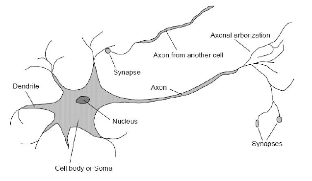
Neurons are the basic elements for information processing. A neuron consists of a cell-body, many dendrites and an axon. The neuron receives electrical signals from other neurons via the dendrites. In the cell-body all input-signals received via the dendrites are accumulated. If the accumulated electrical signal exceeds a certain threshold, the cell-body outputs an electrical signal via it’s axon. In this case the neuron is said to be activated. Otherwise, if the accumulated input at the cell-body is below the threshold, the neuron is not active, i.e. it does not send a signal to connected neurons. The point, where dendrites of neurons are connected to axons of other neurons is called synapse. The synapse consists of an electrochemical substance. The conductivity of this substance depends on it’s concentration of neurotransmitters. The process of learning adapts the conductivity of synapses and, i.e. the degree of connection between neurons. A single neuron can receive inputs from 10-100000 other neurons. However, there is only one axon, but multiple dendrites of other cell can be connected to this axon.
Artificial Neuron#

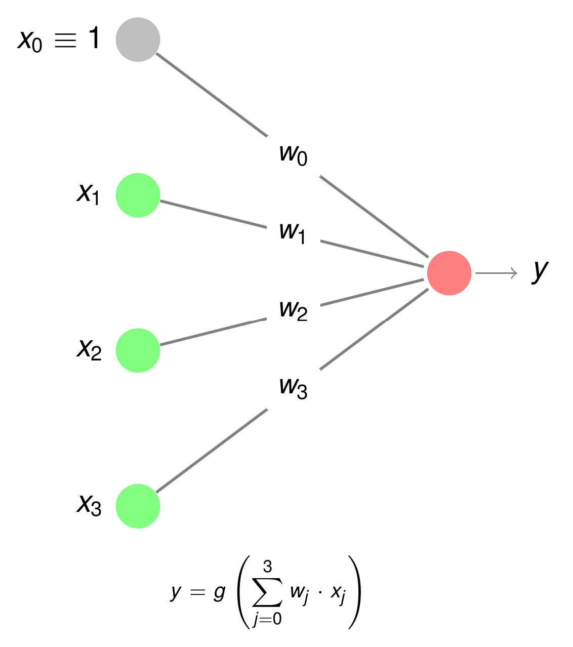
The artificial model of a neuron is shown in the picture below. At the input of each neuron the weighted sum
is calculated. The values \(x_j\) are the outputs of other neurons. Each \(x_j\) is weighted by a scalar \(w_j\), similar as in the natural model the signal-strength from a connected neuron is damped by the conductivity of the synapse. As in the natural model, learning of an artificial network means adaptation of the weights between neurons. Also, as in the natural model, the weighted sum at the input of the neuron is fed to an activation function g(), which can be a simple threshold-function that outputs a 1 if the weighted sum \(in=\sum\limits_{j=0}^d w_jx_j\) exceeds a certain threshold and a 0 otherwise.
Activation Function#
The most common activation functions are:
Threshold:
\[\begin{split}g(in)= \left\lbrace \begin{array}{ll} 1, & in \geq 0 \\ 0, & else \\ \end{array} \right.\end{split}\]Sigmoid:
\[g(in)=\frac{1}{1+exp(-in)}\]Tanh:
\[g(in)=\tanh(in)\]Identity:
\[ g(in)=in \]ReLu:
\[g(in)=max\left( 0 , in \right)\]Softmax:
\[g(in_i,in_j)=\frac{\exp(in_i)}{\sum\limits_{j=1}^{K} \exp(in_j)}\]
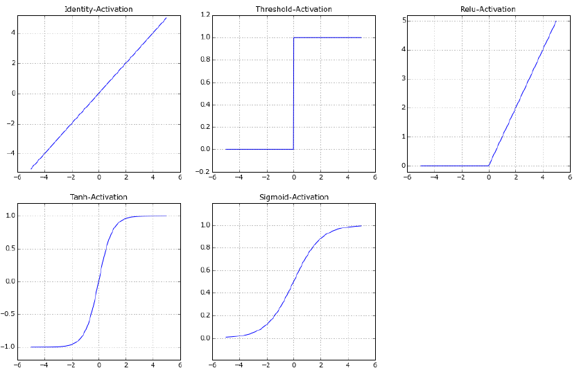
All artificial neurons calculate the sum of weighted inputs \(in\). Neurons differ in the activation function, which is applied on \(in\). In the sections below it will be described how to choose an appropriate activation function.
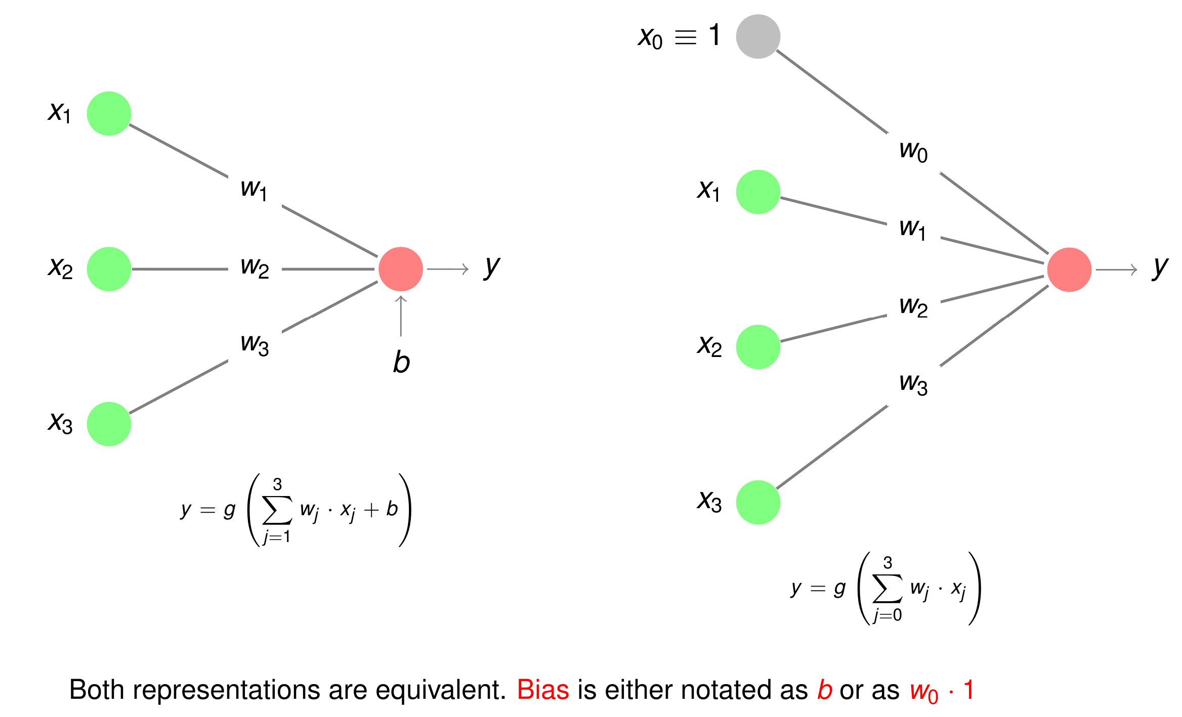
Bias#
Among the input-signals, \(x_0\) has a special meaning. In contrast to all other \(x_j\) the value of this so called bias is constant \(x_0=1\). Instead of denoting the bias input to a neuron by \(w_0 \cdot x_0 = w_0\) it can also be written as \(b\). I.e.
Hence the following two graphical representations are equivalent:
Artificial Neural Networks: General Notions#
Layers#
In Neural Networks neurons are arranged in layers. All Neurons of a single layer are of the same type, i.e. they apply the same activation function on the weighted sum at their input (see previous section). Each Neural Network has at least one input-layer and one output-layer. The number of neurons in the input-layer is determined by the number of features (attributes) in the given Machine-Learning problem. The number of neurons in the output-layer depends on the task. E.g. for binary-classification and regression only one neuron in the output-layer is requried, for classification into \(K>2\) classes the output-layer consists of \(K\) neurons.
Actually, the input-layer is not considered as a real layer, since it only takes in the values of the current feature-vector, but does not perform any processing, such as calculating an activation function of a weighted sum. The input layer is ignored when determining the number of layers in a neural-network.
For example for a binary credit-worthiness classification of customers, which are modelled by the numeric features age, annual income, equity, \(3+1=4\) neurons are required at the input (3 neurons \(x_1,x_2,x_3\) for the 3 features plus the constant bias \(x_0=1\)) and one neuron is required at the output. For non-numeric features at the input, the number of neurons in the inut-layer is not directly given by the number of features, since each non-numeric feature must be One-Hot encoded before passing it to the Neural Network.
Inbetween the input- and the output-layer there may be zero, one or more other layers. The number of layers in a Neural Network is an essential architectural hyperparameter. Hyperparameters in Neural Networks, as well as in all other Machine Learning algorithms, are parameters, which are not learned automatically in the training phase, but must be configured from outside. Finding appropriate hyperparameters for the given task and the given data is possibly the most challenging task in machine-learning.
Feedforward- and Recurrent Neural Networks#
In Feedforward Neural Networks (FNN) signals are propagated only in one direction - from the input- towards the output layer. In a network with \(L\) layers, the input-layer is typically indexed by 0 and the output-layer’s index is \(L\) (as mentioned above the input-layer is ignored in the layer-count). Then in a FNN the output of layer \(j\) can be passed to the input of neurons in layer \(i\), if and only if \(i>j\).
Recurrent Neural Networks (RNN), in contrast to FNNs, not only have forward connections, but also backward-connections. I.e the output of neurons in layer \(j\) can be passed to the input of neurons in the same layer or to neurons in layers of index \(k<j\).
General Concept of Supervised Learning#
Neural Networks can be applied for supervised and unsupervised learning. By far the most applications apply Neural Networks for supervised learning for classification or regression. This notebook only considers this case. Neural Networks for unsupervised learning would be for example Self Organizing Maps, Auto Encoders or Restricted Boltzmann Machines.
The general concept of supervised learning of a neural network is sketched in the picture below.
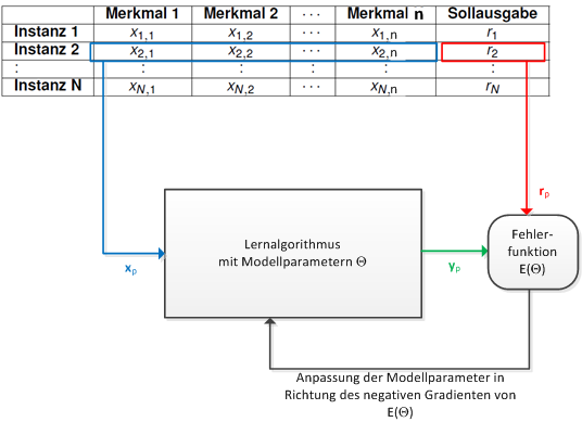
In supervised learning each training element is a pair of input/target. The input contains the observable features, and the target is either the true class-label in the case of classification or the true numeric output value in the case of regression. A Neural Network is trained by passing a single training-element to the network. For the given input the output of the network is calculated, based on the current weight values. This output of the network is compared with the target. As long as there is a significant difference between the output and the target, the weights of the networks are adapted. In a well trained network, the deviation between output and target is as small as possible for all training-elements.
Gradient Descent Learning#
In the previous section the general idea of training a Neural Network has been presented. Now, a concrete realization of this concept is described - Gradient Descent - and Stochastic Gradient Descent Learning. This approach is not only applied for all types of Neural Networks, but for many other supervised Machine Learning algorithms.
Gradient Descent Learning#
The concept of Gradient Descent Learning is as follows:
Define a Loss Function \(E(T,\Theta)\), which somehow measures the deviation between the current network \(\mathbf{y}\) output and the target output \(\mathbf{r}\). As above,
is the set of labeled training data and
is the set of parameters (weights), which are adapted during training. 2. Calculate the gradient of the Loss Function:
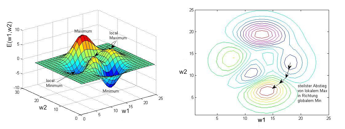
The gradient of a function points towards the steepest ascent of the function at the point, where it is calculated. The negative gradient \(-\nabla E(T,\Theta)\) points towards the steepest descent of the function. 3. Adapt all parameters into the direction of the negative gradient. This weight adaptation guarantees that the Loss Function is iteratively minimized.:
where \(\eta\) is the important hyperparameter learning rate. The learning rate controls the step-size of weight adaptations. A small \(\eta\) implies that weights are adapted only slightly per iteration and the learning algorithm converges slowly. A large learning-rate implies strong adaptations per iteration. However, in this case the risk of jumping over the minimum is increased. Typical values for \(\eta\) are in the range of \([0.0001,0.1]\).
Below, the calculation of
for regression, binary and non-binary classification is presented.-
Single Layer Perceptron#
A Single Layer Perceptron (SLP) is a Feedforward Neural Network (FNN), which consists only of an input- and an output layer (the output-layer is the single layer). All neurons of the input layer are connected to all neurons of the output layer. A layer with this property is also called a fully-connected layer or a dense layer. SLPs can be applied to learn
a linear binary classifier
a linear classifier for more than 2 classes
a linear regression model
SLP for Regression#
A SLP can be applied to learn a linear function
from a set of N supervised observations
where \(x_{j,t}\) is the j.th feature of the t.th training-element and \(r_t\) is the numeric target value of the t.th training-element.
As depicted above, for linear regression only a single neuron in the output-layer is required. The activation function \(g()\) applied for regression is the identity function. The loss-function, which is minimized in the training procedure is the sum of squared error:
where \(\Theta=\lbrace w_0,w_1,\ldots, w_d \rbrace\) is the set of weights, which are adapted in the training process.
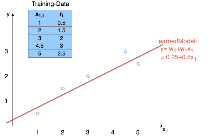
Example: The \(N=5\) training-elements given in the table of the picture below contain only a single input feature \(x_1\) and the corresponding target-value \(r\). From these training-elements a SLP can learn a linear function \(y=w_0+w_1 x_1\), which minimizes the loss-function SSE.
SLP for binary classification#
A SLP can be applied to learn a binary classifier from a set of N labeled observations
where \(x_{j,t}\) is the j.th feature of the t.th training-element and \(r_t \in \lbrace 0,1 \rbrace\) is the class-index of the t.th training-element.
As depicted above, for binary classification only a single neuron in the output-layer is required. The activation function \(g()\) applied for binary classification is either the threshold- or the sigmoid-function. The threshold-function output values are either 0 or 1, i.e. this function can provide only a hard classifikcation-decision, with no further information on the certainty of this decision. In contrast the value range of the sigmoid-function covers all floats between 0 and 1. It can be shown that if the weighted-sum is processed by the sigmoid-function the output is an indicator for the a-posteriori propability that the given observation belongs to class \(C_1\):
If the output value
is larger than 0.5 the observation \((x_{1},x_{2}, \ldots,x_{d})\) is assigned to class \(C_1\), otherwise it is assigned to class \(C_0\). A value close to 0.5 indicates an uncertaion decision, whereas a value close to 0 or 1 indicates a certain decision.
In the case that the sigmoid-activation function is applied, the loss-function, which is minimized in the training procedure is the binary cross-entropy function:
where \(r_t\) is the target class-index and \(y_t\) is the output of the sigmoid-function, for the t.th training-element. Again, \(\Theta=\lbrace w_0,w_1,\ldots, w_d \rbrace\) is the set of weights, which are adapted in the training process.
Example: The \(N=9\) 2-dimensional labeled training-elements given in the table of the picture below are applied to learn a SLP for binary classification. The learned model can be specified by the parameters (weights)
These weights define a line
whose slope is
and whose intersection with the \(x_2\)-axis is
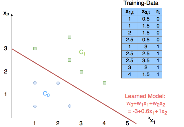
Once this model, i.e. the set of weights, is learned it can be applied for classification as follows: A new observation \(\mathbf{x'}=(x'_1,x'_2)\) is inserted into the learned equation \(w_0 \cdot 1 + w_1 \cdot x'_1 + w_2 \cdot x'_2\). The result of this linear equation is passed to the sigmoid-function. If sigmoid-function’s output is \(>0.5\) the most probable class is \(C_1\), otherwise it is \(C_0\).
SLP for classification in \(K>2\) classes#
A SLP can be applied to learn a non-binary classifier from a set of N labeled observations
where \(x_{j,t}\) is the j.th feature of the t.th training-element and \(r_t \in \lbrace 0,1 \rbrace\) is the class-index of the t.th training-element.
As depicted above, for classification into \(K>2\) classes K neurons are required in the output-layer. The activation function \(g()\) applied for non-binary classification is usually the softmax-function:
The softmax-function outputs for for each neuron in the output-layer a value \(y_k\), with the property, that
Each of these outputs is an indicator for the a-posteriori propability that the given observation belongs to class \(C_i\):
The class, whose neuron outputs the maximum value is the most likely class for the current observation at the input of the SLP.
In the case that the softmax-activation function is applied, the loss-function, which is minimized in the training procedure is the cross-entropy function:
where \(\Theta=\lbrace w_0,w_1,\ldots, w_d \rbrace\) is the set of weights, which are adapted in the training process. \(r_{t,k}=1\), if the t.th training-element belongs to class \(k\), otherwise it is 0. \(y_{t,k}\) is the output of the k.th neuron for the t.th training-element.
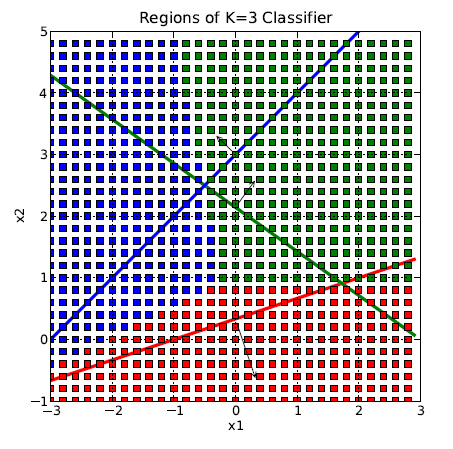
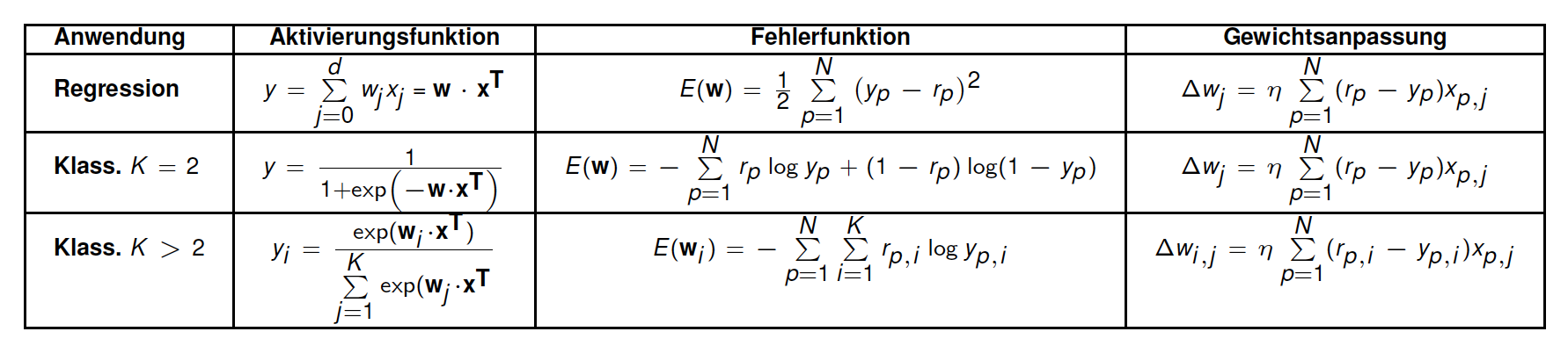
Each output neuron has its own set of weights, and each weight-set defines a (d-1)-dimensional hyperplane in the d-dimensional space. However, now these hyperplanes are not the class boundary itself, but they determine the class boundaries, which are actually of convex shape as depicted below. In the picture below, the red area indicates the inputs, who yield a maximum output at the neuron, whose weights belong to the red line, the blue area is the of inputs, whose maximum value is at the neuron, which belongs to the blue line and the green area comprises the inputs, whose maximum value is at the neuron, which belongs to the green line.
Gradient of Error Function#
Above, the general idea of Gradient Descent Learning has been described. The corresponding weight-adaptation rule is:
Now, we know which loss-function \(E(T,\Theta)\) is applied for the 3 different cases. Hence, we can calculate for each of these loss-functions the value of
Even though different loss functions are applied, the gradient calculation of the loss-function yields the same weight-adaptation for all of the 3 mentioned cases:
for all \(i \in [1,K]\) and \(j \in [0,d]\) (\(K\) is the number of neurons in the output-layer). The difference between target- and network output at the i.th neuron of the t.th training-element is also called the error-signal
and the error-vector comprises the error signals at all \(K\) output-neurons for the t.th training-element:
With this notation the simultaneous adaptation of all weights in \(W\) can be calculated as follows:
with
Note that \(\boldsymbol{\Delta}_t\) is a column vector and \(\boldsymbol{x}_{t}^T\) is a row-vector. Hence, the resulting matrix-product \(\boldsymbol{\Delta}_t \boldsymbol{x}_{t}^T\) has as much rows as there are rows in \(\boldsymbol{\Delta}_t\) and as much columns as there are columns in \(\boldsymbol{x}_{t}^T\).
This calculation of the weight-adaption from the error-vector at the output of the neural network is also called the Backward-Pass.
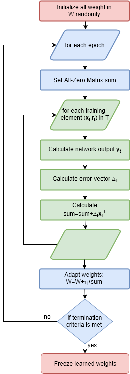
As can be seen in this weight-adaptation formula, for each single adaptation the entire batch of \(N\) training-elements is regarded (since the sum goes over all training-elements). This is called Batch-Learning. The flowchart of the described Gradient Descent Learning is depicted below. In the context of Neural Network training an epoch means that each element of the entire training-dataset has been shown used once for weight-adaptation. Usually, the entire training-process comprises many epochs. The termination of the training-process is either defined by a fixed number of epochs, or by a threshold on the decrease of the Loss Function. I.e. if the loss does not decrease significantly over several iterations, training terminates.
Stochastic Gradient Descent Learning#
A quite popular variant of the Gradient Descent Batch-Learning is to regard for a single weight-adaptation only a single training element. In this variant the weight adaptation with respect to the t.th training-element is:
In contrast to Batch-Learning this variant is called Online-Learning. The true Gradient Descent approach would require Batch-Learning. Since the Online-Learning variant is not fully conform to the Gradient Descent approach it is called Stochastic Gradient Descent (SGD).
Summary Single Layer Perceptron#
Multi Layer Perceptron#
Notations and Basic Characteristics#
A Multi Layer Perceptron (MLP) with \(L\geq 2\) layers is a Feedforward Neural Network (FNN), which consists of
an input-layer (which is actually not counted as layer)
an output layer
a sequence of \(L-1\) hidden layers inbetween the input- and output-layer
Usually the number of hidden layers is 1,2 or 3. All neurons of a layer are connected to all neurons of the successive layer. A layer with this property is also called a fully-connected layer or a dense layer.
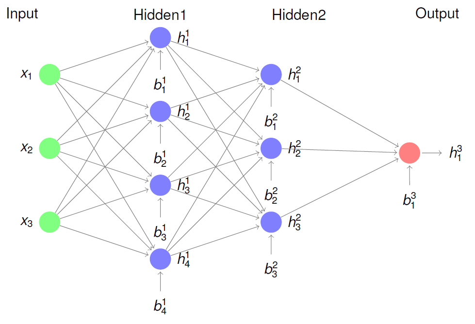
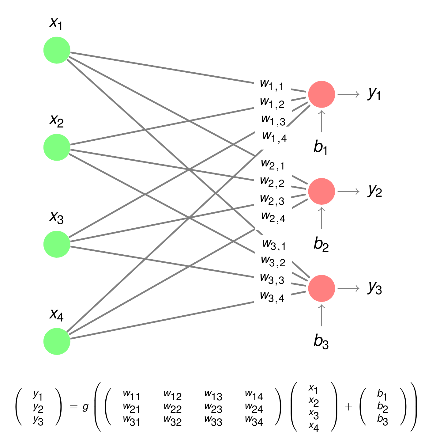
An example of a \(L=3\) layer MLP is shown in the following picture.
As in the case of SLPs, the biases in MLP can be modelled implicitily by including to all non-output-layers a constant neuron \(x_0=1\), or by the explicit bias-vector \(\mathbf{b^l}\) in layer \(l\). In the picture above, the latter option is applied.
In order to provide a unified description the following notation is used:
the number of neurons in layer \(l\) is denoted by \(z_l\).
the output of the layer in depth \(l\) is denoted by the vector \(\mathbf{h^l}=(h_1^l,h_2^l,\ldots,h_{z_l}^l)\),
\(\mathbf{x}=\mathbf{h^0}\) is the input to the network,
\(\mathbf{y}=\mathbf{h^L}\) is the network’s output,
\(\mathbf{b^l}\) is the bias-vector of layer \(l\),
\(W^l\) is the weight-matrix of layer \(l\). It’s entry \(W_{ij}^l\) is the weight from the j.th neuron in layer \(l-1\) to the i.th neuron in layer \(l\). Hence, the weight-matrix \(W^l\) has \(z_l\) rows and \(z_{l-1}\) columns.
With this notation the Forward-Pass of the MLP in the picture above can be calculated as follows:
Output of first hidden-layer:
Output of second hidden-layer:
Output of the network:
As in the case of Single Layer Perceptrons the three categories
regression,
binary classification
\(K\)-ary classification
are distinguished. The corresponding MLP output-layer is the same as in the case of a SLP.
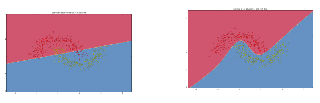
In contrast to SLPs, MLPs are able to learn non-linear models. This difference is depicted below: The left hand side shows the linear classification-boundary, as learned by a SLP, whereas on the right-hand side the non-linear boundary, as learned by a MLP from the same training data, is plotted.
Architecture#
Activation- and Loss-functions#
Activation functions in the output layer and loss functions#
The configuration of the activation function in the output-layer and the loss function, which is minimized in the training-stage, depend on the application-category in the same way as in the SLP:
Regression:
Number of neurons in the output-layer: 1
Activation function in the output-layer: identity
Loss Function: Sum of Squared Errors (SSE)
Binary Classification:
Number of neurons in the output-layer: 1
Activation function in the output-layer: sigmoid
Loss Function: binary Cross-Entropy
\(K\)-ary Classification:
Number of neurons in the output-layer: K
Activation function in the output-layer: softmax
Loss Function: Cross-Entropy
Gradient Descent Learning#
For training, MLPs apply the same approach as SLPs: Gradient Descent. The general consept of Gradient Descent learning is:
Define a Loss Function \(E(T,\Theta)\), which somehow measures the deviation between the current network \(\mathbf{y}\) output and the target output \(\mathbf{r}\).
Calculate the gradient of the Loss Function:
Adapt all parameters into the direction of the negative gradient. This weight adaptation guarantees that the Loss Function is iteratively minimized.:
where \(\eta\) is the important hyperparameter learning rate.
For the MLP, here we just present the Backward Pass weight adaptation-rule, resulting from the aforementioned Gradient Descent approach. The algorithm is denoted Backpropagation Algorithm.
The weight-matrix \(W^l\) in layer \(l\), with \(l \in \lbrace 1,\ldots,L\rbrace\), is adapted in each iteration by
where
for Gradient Descent Batch-Learning, and
for Stochastic Gradient Descent (SGD) Online-Learning. In this adaptation formulas
\(\mathbf{h}_t^{l-1}\) is the output-vector at layer \(l-1\), if the t.th training-element \(\mathbf{x}_t\) is at the input of the MLP,
the matrix \(\boldsymbol{D}_t^l\) is calculated recursively as follows:
where:
\(*\) denotes matrix-multiplication
\(\cdot\) denotes elementwise-multiplication
\(g'()\) is the first derivation of the activation function applied in layer \(l\).
the error-vector \(\Delta_t\) is as defined in notebook SLP:
Note that in the calculation of \(\boldsymbol{D}_t^l\) depends on the weight-matrices \(W^{l+1},\ldots W^{L}\). It is important that for this the old weight-matrices (before the update in the current iteration) are used.
Hyperparameters#
In the previous sections the following Neural Network hyperparameters, i.e. parameters, which must be configured and optimized by the user, have been mentioned:
Number of layers L in the network: For SLP this is fixed to \(L=1\).
Number of neurons per layer: For the input layer this number is given by the number of features and for the output-layer this number is given by the task (regression, binary classification or \(K\)-ary classification). Since in SLPs there are no other layers, the number of neurons per layer is actually fixed.
Activation function g(): For the 3 different tasks (regression, binary classification or \(K\)-ary classification), the most convenient activation functions in the neurons of the output-layer have been described above. However, others are possible.
Learning Parameters:
Batch- or Online-Learning
The learning rate \(\eta\) is a very sensitive parameter, which must be selected carefully.
Learning termination criteria and maximum number of epochs
Actually, there are many variants of Gradient Descent and Stochastic Gradient Descent, e.g. Backpropagation, RMSprop, Adam, …
There are more crucial hyperparameters, which are shortly described here:
Learnrate Decay \(\gamma\): If a learnrate decay of \(\gamma \lt 1\) is selected the learnrate \(\eta\) is decreased after each epoch as follows:
where \(l-1\) and \(l\) indicate the previous and current epoch, respectively.
Momentum \(\alpha\): In order to avoid a ping-ponging of weight adaptations the previous weight adaptation is integrated into the current weight-adaptations as follows:
Here, the superscripts \(l-1\) and \(l\) indicate the previous and current weight adaptations, respectively.
Weight Decay \(\beta\): Different loss functions \(E(T,\Theta)\) have been presented above. In the case of weight-decay, i.e. \(\beta \gt 0\) an additional term
is added to the loss function. Then for this extended loss function the gradient is calculated and weights are adapted into the direction of the negative gradient of the extended loss-function. The effect is, that then the error-signals and the weights are minimized simultaneously. Small weight values reduce the risk of overfitting. However, too small weights may yield too simple models (underfitting). The extend of weight-minimization can be controlled by the value of \(\beta\). This process is also called Regularization. It is applied not only for Neural Networks, but in many other Machine Learning algorithms.
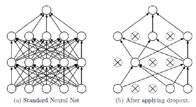
Dropout: Dropout is a technique to prevent Neural Networks, such as MLPs, CNNs, LSTMs from overfitting. The key idea is to randomly drop units along with their connections from the neural network during training. This prevents units from co-adapting too much. The drop of a defined ratio (0.1-0.5) of random neurons is valid only for one iteration. During this iteration the weights of the droped units are not adapted. In the next iteration another set of units, which are dropped temporarily is randomly selected. Dropout is only applied in the training-phase.
Early MLP Example: Autonomos Driving#
The ALVINN net is a MLP with one hidden layer. It has been designed and trained for road following in autonomous driving. The input has been provided by a simple \(30 \times 32\) greyscale camera. As shown in the picture below, the hidden layer contains only 4 neurons. In the output-layer each of the 30 neurons belongs to one “steering-wheel-direction”. The training data has been collected by recording videos while an expert driver steers the car. For each frame (input) the steering-wheel-direction (label) has been tracked.
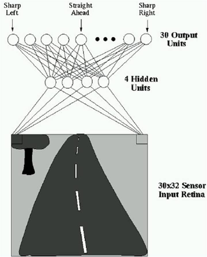
After training the vehicle cruised autonomously for 90 miles on a highway at a speed of up to 70mph. The test-highway has not been included in the training cruises.