
Recurrent Neural Networks
Contents
Recurrent Neural Networks#
Author: Johannes Maucher
Last Update: 30.10.2020
Recap: Feedforward Neural Networks#
Feedforward neural networks have already been introduced in 01NeuralNets.ipynb. Here, we just repeat the basics of feedforward nets in order to clarify how Recurrent Neural Networks differ from them.
In artificial neural networks the neurons are typically arranged in layers. There exist weighted connections between the neurons in different layers. The weights are learned during the training-phase and define the overall function \(f\), which maps an input-signal \(\mathbf{x}\) to an output \(\mathbf{y}\). In a feed-forward network the neural layers are ordered such that the signals of the input-neurons are connected to the input of the neurons in the first hidden layer. The output of the neurons in the \(i.th\) hidden layer are connected to the input of the neurons in the \((i+1).th\) hidden layer and so on. The output of the neurons in the last hidden layer, are connected to the neurons in the output layer. In particular there are no backward-connections in a feed-forward network. A multilayer-perceptron (MLP) is a feed-forward network in which all neurons in layer \(i\) are connected to all neurons in layer \(i+1\). A simple MLP with 3 input neurons, one hidden layer and one neuron in the output layer is depicted in figure below.

The picture below contains another representation of the MLP, which hides the details of the topology, while emphasizing the algebraic operations:

If the output of the neurons in layer \(k\) are denoted by
the input to the network is \(\mathbf{h}^0=\mathbf{x}\) and the bias values of the \(z_k\) neurons in layer \(k\) are arranged in the vector
then the output at each layer \(k\) can be calculated by
where \(g(\cdot)\) is the activation-function. Typical activation-functions are e.g. sigmoid-, tanh-, softmax- or the identity-function. The weight matrix \(W^k\) of layer \(k\) consists of \(z_k\) rows and \(z_{k-1}\) columns. The entry \(W_{ij}^k\) in row \(i\), column \(j\) is the weight of the connection from neuron \(j\) in layer \(k-1\) to neuron \(i\) in layer \(k\).
Recurrent Neural Networks#
In feed-forward neural networks the output depends only on the network parameters and the current input vector. Previous or successive input-vectors are not regarded. This means, that feed-forward networks do not model correlations between successive input-vectors.
E.g. in Natural Language Processing (NLP) the input signals are often words of a phrase, sentence, paragraph or document. Obviously, successive words are correlated. Speech and text are not the only domains of correlated data. For all time-series-data, e.g. temperature, stock-market, unemployment-numbers, …we also have temporal correlations. A feed-forward network would ignore these correlations. Recurrent Neural Networks (RNNs) would be better for this type of data.
The architecture of a simple recurrent layer is depicted in the figure below. RNNs operate on variable-length sequences of input. In contrast to simple feedforward-networks, they have connections in forward- and backward-direction. The backward-connections realise an internal state, or memory. In each time stamp the output \(h^1(t)\) is calculated in dependence of the current input \(x(t)\) and the previous output \(h^1(t-1)\). Thus the current output depends on the current input and all former outputs. In this way RNNs model correlations between successive input elements.


The recurrent-layer’s output \(\mathbf{h}^1(t)\) from the current input \(\mathbf{x}(t)\) and the previous output \(\mathbf{h}^1(t-1)\), can equivalently be realized by a single matrix multiplication, if the weight matrices \(W^1 \) and \(R^{1}\) are stacked horizontally and the column-vectors \(\mathbf{x}(t)\) and \(\mathbf{h}^1(t-1)\) are stacked vertically:
For simple recurrent layers of this type, typically the tanh activation function is applied.
The picture above depicts a single recurrent layer. In a (deep) neural network several recurrent layers can be stacked togehter. A convenient architecture-type for sequence-classification (e.g. text-classification) contains one or more recurrent layers and one or more dense layers at the output. In this constellation the dense layers at the output serve as classifier and the recurrent layers at the input generate a meaningful representation of the input-sequence. However, sequence-classification (many-to-one) is only one application category of recurrent neural networks. Other categories are described in subsection Application Categories.
Application Categories of Recurrent Neural Networks#
In order to distinguish RNN application categories we apply an abstract representations of neural networks in which
the input \(\mathbf{x}\) is represented by a green rectangle.
the output \(\mathbf{h}^k\) of a (recurrent) hidden-layer is represented by a purple rectangle.
the output of the network \(\mathbf{y}=\mathbf{h}^L\) is represented by a red rectangle.
Moreover, without loss of generality, only networks with a single (recurrent) hidden layer are considered here.
One-to-One (Feedforward Neural Network)#
With the notation defined above a Feedworward Neural Network with one hidden layer is abstractly defined as below:

This type of model represents the standard supervised learning algorithms for classification and regression, where all input-vectors are considered to be independent of each other.
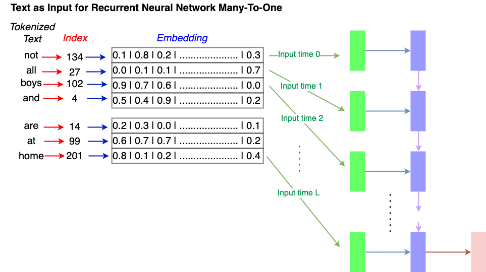
Many-to-One (RNN)#
A many-to-one recurrent architecture maps a sequence of input-vectors to a single output. An example for this category is text-classification, where each input represents a single word and a class-label must be calculated for the entire sequence. At each time stamp \(t \in [1,T]\)
a new input-vector \(x(t)\) (word representation) is passed to the net
a new hidden-state \(h(t)\) is calculated in dependence of \(x(t)\) and the previous hidden-state \(h(t-1)\)
At the end of the sequence the network output \(y\) is calculated from the hidden-state \(h(T)\).

Examples:

Many-to-Many (RNN)#
A many-to-many recurrent architecture maps a sequence of input-vectors to a sequence of output-vectors. An example for this category is language-translation, where each input represents a single word. The entire sequence is usually a sentence and the output is the translated sentence. At each time stamp \(t \in [1,T]\)
a new input-vector \(x(t)\) (word representation) is passed to the net
a new hidden-state \(h(t)\) is calculated in dependence of \(x(t)\) and the previous hidden-state \(h(t-1)\)
At each time stamp \(t' \in [1+d,T+d]\)
a new output-vector \(y(t')\) is calculated from the hidden-state \(h(t')\). For \(t'>T\), the hidden-state \(h(t')\) is calculated only from \(h(t'-1)\).
The parameter \(d\) describes the delay between the input and the output sequence. In language translation usually \(d>0\), i.e the first word of the translation is calculated not before the first \(d\) words of the sentence in the source-language have been passed do the network.

The case, where \(d>0\) is called the asynchronous case (picture above). The synchronous many-to-many case is defined by \(d=0\) (picture below). A application of this category is e.g. frame-by-frame labeling of a video-sequence.

One-To-Many (RNN)#
Finally, the one-to-many recurrent architecture maps a single vector at the input, to a sequence of output-vectors. A concrete application of this category is image-captioning, where the input is a single image, and the output is a sequence of words, which describes the contents of the image in a natural language. As can be seen in the picture below, the input \(x(t=1)\) is applied to calculate the first hidden-state \(h(t=1)\). All following hidden states \(h(t)\) are calculated only from \(h(t-1)\). For each hidden-state \(h(t)\) a corresponding output \(y(t)\) is calculated.

Bidirectional RNN#
A bidirectional RNN calculates two types of hidden-states at it’s output:
The first type is the same as described up to now in this notebook. I.e. the current recurrent hidden layer output \(h^1(t)\) is calculated from the current input \(x(t)\) and the recurrent hidden output from the previous time-step \(h^1(t-1)\).
The second type calculates recurrent hidden states in the backward direction. I.e the current recurrent hidden layer output \(h'^1(t)\) is calculated from the current input \(x(t)\) and the recurrent hidden output from the next time-step \(h'^1(t+1)\).

The output of the network is then calculated from both hidden states \(h^1(t)\) and \(h'^1(t)\). In this way not only dependencies from previous inputs, but also from future inputs is taken into account. This is particular helpful in Natural Language Processing tasks, where inputs are successive words.
Bidirectional RNNs are implemented by stacking together two RNN-layer modules, where each layer can be of any RNN-type, e.g. simple RNN, LSTM or GRU.
Long-short-Term-Memory (LSTM) networks#
Simple RNNs, as described and depicted in Simple RNN, suffer from an important problem: Applying Stochastic Gradient Descent allows to learn short-term dependencies quite well, but the network is not capable to learn long-term dependencies. The reason for this drawback is the vanishing gradient problem: In SGD weights are updated proportional to the gradient of the loss-function with respect to the specific weight. In some areas of the networks these gradients get marginal, i.e. the weights are not adapted any longer. S. Hochreiter and J. Schmidhuber studied the problem of vanishing gradients in simple RNNs in their famous paper Long short-term Memory and they proposed a new type of RNN, which circumvents this problem and is able to learn also long-term dependencies. The architecture of such a Long short-term Memory Network (LSTM) is depicted below:

As shown in the figure above a LSTM keeps and updates a so called cell-state. This cell-state mainly realises the memory. The network is able to learn, which parts in the memory (cell-state) can be forgotten and which parts of the memory shall be updated. The new hidden-state \(h^1(t)\) depends not only on the previous hidden state \(h^1(t-1)\) and the current input \(x(t)\), but also on the memory (cell-state).
The forget-gate outputs a filter \(f(t)\) which determines the information of the memory (cell-state), that can be forgotten. The second gate outputs \(i(t)\), which determines which parts of the memory shall be updated and the output \(\underline{C}(t)\) determines how this update shall look like. The last gate at the bottom defines how the hidden-state shall be updated in dependance of the current input, the previous hidden state \(h^1(t-1)\) the new cell-state (memory).
Since LSTMs are a special kind of RNNs, all application-categories, described in subsection RNN application categories are also applicable for them.
Gated Recurrent Unit (GRU)#
Recurrent Neural Networks with Gated Recurrent Unit (GRU) have been introduced in Cho et al: On the Properties of Neural Machine Translation: Encoder–Decoder Approaches. They perform as well as LSTMs on sequence modelling, while being conceptually simpler. As shown in the figure below, similar to the LSTM unit, the GRU has gating units that modulate the flow of information inside the unit, however, without having a separate cell-state memory. The output of the GRU \(h^1(t)\) is a linear interpolation of the previous output \(h^1(t-1)\) and a candidate output \(\underline{h}^1(t)\). The weighting of these two elements is defined by the update-filter \(i(t)\). The output \(f(t)\) of the forget-gate determines which parts from the previous hidden state \(h^1(t-1)\) can be forgotten in the calculation of the candidate output \(\underline{h}^1(t)\).

An empirical evaluation of LSTMs and GRUs can be found in Chung et al, Empirical Evaluation of Gated Recurrent Neural Networkson Sequence Modeling.