.ipynb .pdf

Binder

Contents

Gaussian and Difference of Gaussian Pyramid

• Author: Johannes Maucher

• Last Update: 28th January 2021

In the previous sections two important applications of Gaussian filters, bluring and noise suppression, have been introduced. Another frequent application is to construct Gaussian and Laplacian pyramides. Pyramides are used to generate different sizes of an images. The levels in a pyramid differ in their scale. Different scales are required for example for implementing scale-invariant recognition. This will be elaborated in detail in the later section on SIFT features.

A Gaussian pyramide is constructed as follows:

1. Set level index \(l=0\); Set \(G_{l=0}\) to be the original image

2. Smooth \(G_l\) by applying a Gaussian filter

3. Downsample the smoothed \(G_l\) by a factor of 2. The result is \(G_{l+1}\)

4. Set \(l=l+1\) and continue with step 2 until \(G_l\) contains only a single pixel

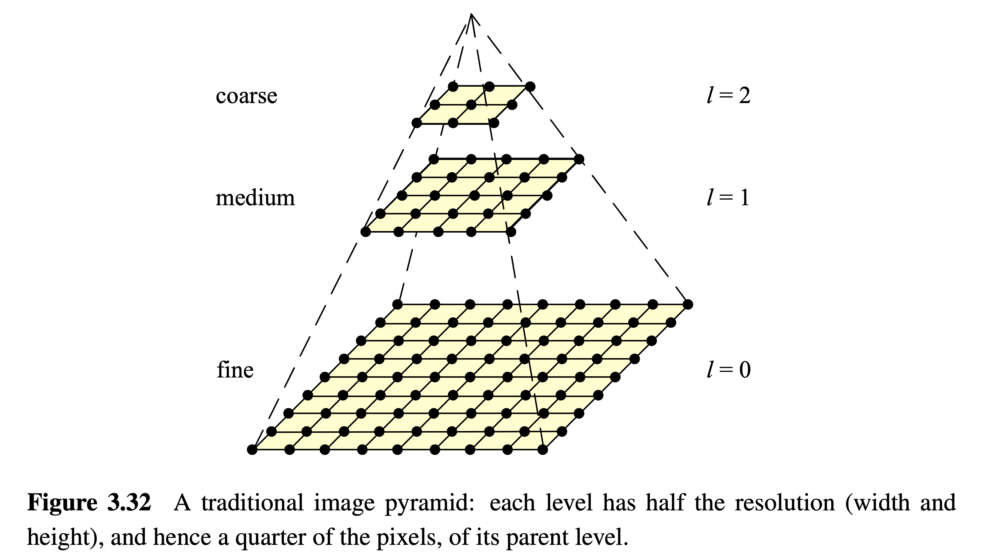
Image Source: [Sze10]

In the Gaussian pyramid in each level the input image is low pass filtered. Thus in each level finer structures (higher frequencies) are filtered out. At high levels \(l\) only coarse structures (low frequencies) are represented in \(G_l\). The Difference at level \(l\)

\[ D_l=G_l-G_{l+1}^{\uparrow} \]

represents the high frequencies which are filtered out in level \(l\), where \(G_{l+1}^{\uparrow}\) is the upsampled (interpolated) version of \(G_{l+1}\). The pyramide of all \(D_l\) constitute the Laplacian Pyramid.

Image Source: [Sze10]

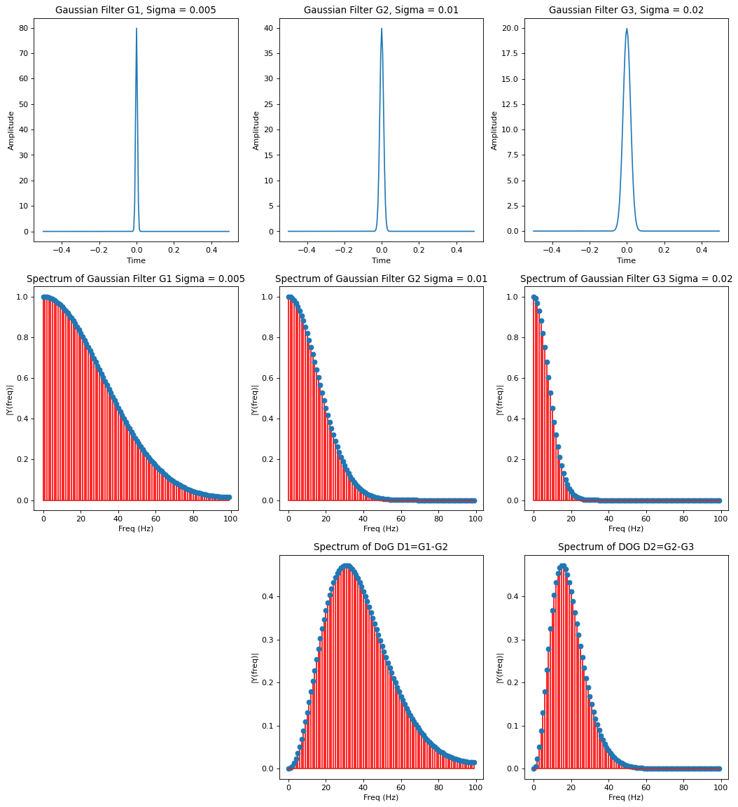
Spectrum of 1-dimensional Gaussian and Difference Of Gaussian Filter

Below the spectrum of

• the 3 different 1-dimensional Gaussian filters \(G_{0}, G_{1}\) and \(G_{2}\)

• the Difference of Gaussian (DoG) \(D_1=G_1-G_{2}^{\uparrow}\) and \(D_2=G_2-G_{3}^{\uparrow}\)

is plotted:

%matplotlib inline
from matplotlib import pyplot as plt
import numpy as np
import scipy.fft as sf
import scipy.ndimage as ndi
import warnings
warnings.filterwarnings("ignore")

Function for calculating and plotting the spectral representation of a signal:

The function below calculates the single-sided amplitude spectrum of a 1-dimensional time domain signal \(y\). The sampling frequency \(Fs\) is required for a correct scaling of the frequency-axis in the plot.

def plotSpectrum(y,Fs,title=""):
 """
 Plots a Single-Sided Amplitude Spectrum of y(t)
 """
 n = len(y) # length of the signal
 k = np.arange(n)
 T = n/Fs
 frq = k/T # two sides frequency range
 frq = frq[range(int(n/2))] # one side frequency range

 Y = sf.fft(y)/n # fft computing and normalization
 Y = Y[range(int(n/2))]

 plt.stem(frq,abs(Y),'r') # plotting the spectrum
 plt.title(title)
 plt.xlabel('Freq (Hz)')
 plt.ylabel('|Y(freq)|')

Define 1-dimensional Gaussian filter:

def calcGaussian(x,m,sig):
    return np.exp(-((tf-m)/sig)**2/2)/(sig*np.sqrt(2*np.pi))

Plot signal, filter and filtered signal in time- and frequency domain:

Fs = 200.0;  # sampling rate
Ts = 1.0/Fs; # sampling interval
tf=np.arange(-0.5,0.5,Ts) # time vector for filter
filtTitle="Gaussian Filter"
sig=0.005
m=0.0

plt.figure(num=None, figsize=(16,18), dpi=80, facecolor='w', edgecolor='k')
plt.subplot(3,3,1)
filt1=calcGaussian(tf,m,sig)
plt.plot(tf,filt1)
plt.title(filtTitle + " G1, Sigma = "+str(sig))
plt.xlabel('Time')
plt.ylabel('Amplitude')
ymargin=0.05
ymin,ymax=plt.ylim()
plt.ylim(ymin-ymargin,ymax+ymargin)
plt.subplot(3,3,2)
filt2=calcGaussian(tf,m,2*sig)
plt.plot(tf,filt2)
plt.title(filtTitle + " G2, Sigma = "+str(2*sig))
plt.xlabel('Time')
plt.ylabel('Amplitude')
ymargin=0.05
ymin,ymax=plt.ylim()
plt.ylim(ymin-ymargin,ymax+ymargin)
plt.subplot(3,3,3)
filt3=calcGaussian(tf,m,4*sig)
plt.plot(tf,filt3)
plt.title(filtTitle + " G3, Sigma = "+str(4*sig))
plt.xlabel('Time')
plt.ylabel('Amplitude')
ymargin=0.05
ymin,ymax=plt.ylim()
plt.ylim(ymin-ymargin,ymax+ymargin)

plt.subplot(3,3,4)
plotSpectrum(filt1,Fs,title="Spectrum of "+filtTitle+ " G1 Sigma = "+str(sig))
plt.subplot(3,3,5)
plotSpectrum(filt2,Fs,title="Spectrum of "+filtTitle+ " G2 Sigma = "+str(2*sig))
plt.subplot(3,3,6)
plotSpectrum(filt3,Fs,title="Spectrum of "+filtTitle+ " G3 Sigma = "+str(4*sig))
plt.subplot(3,3,8)
plotSpectrum(filt2-filt1,Fs,title="Spectrum of DoG D1=G1-G2")
plt.subplot(3,3,9)
plotSpectrum(filt3-filt2,Fs,title="Spectrum of DOG D2=G2-G3")

Gaussian Pyramide and Laplacian Pyramide of Images

Below the Gaussian- and the Laplacian Pyramide of a given image is calculated and visualized. For the calculations of the pyramids the functions pyramid_gaussian() and pyramid_laplacian() from scikit-image are applied.

#!conda install -y scikit-image

from skimage.transform.pyramids import pyramid_gaussian, pyramid_laplacian
import cv2
from matplotlib import pyplot as plt

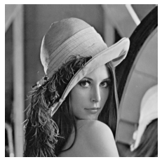
image = cv2.imread('../Data/lenaGrey.png',cv2.IMREAD_GRAYSCALE)
lenaGrey=image.copy()
plt.axis("off")
plt.imshow(image,cmap="gray")
plt.show()

Calculate Gaussian- and Laplacian Pyramide:

MAXlevel=4
gausspyramid=tuple(pyramid_gaussian(image, max_layer=MAXlevel, downscale=2, sigma=None, order=1, mode='reflect', cval=0))
laplacianpyramid=tuple(pyramid_laplacian(image, max_layer=MAXlevel, downscale=2, sigma=None, order=1, mode='reflect', cval=0))

Visualize the pyramids:

titles=["Original",
        "Diff between Original and Smoothed 1",
        "Smoothed 1",
        "Diff between Smoothed 1 and Smoothed 2",
        "Smoothed 2",
        "Diff between Smoothed 2 and Smoothed 3",
        "Smoothed 3",
        "Diff between Smoothed 3 and Smoothed 4",
       ]

idx=1
plt.figure(figsize=(14,24))
for level in range(MAXlevel):
    plt.subplot(MAXlevel,2,idx)
    plt.imshow(gausspyramid[level],cmap="gray")
    plt.title(titles[idx-1])
    idx+=1
    plt.subplot(MAXlevel,2,idx)
    plt.imshow(laplacianpyramid[level],cmap="gray")
    plt.title(titles[idx-1])
    idx+=1

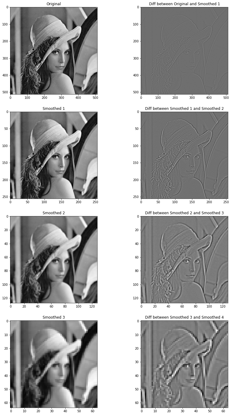
In the left column of the picture above the Gaussian pyramide, in the right column the Laplacian pyramide is shown (both upsidedown).

Noise Suppression Global Image Features