
Object Detection
Introduction
Goal
The goal of object detection is to dermine for a given image:
Which objects are in the image
Where are these objects
Confidence score of detection

Approaches
An old approach for obect detection is sliding window detection. Here a window is slided over the entire image. For each window a classifier determines, which object is contained in the window. In the most simple version only one object-type (e.g. car) is of interest and the binary classifier has to distinguish if this object is contained in the window or not. The corresponding position information provided implicitely by the position of the current window within the image. This approach is depicted below:
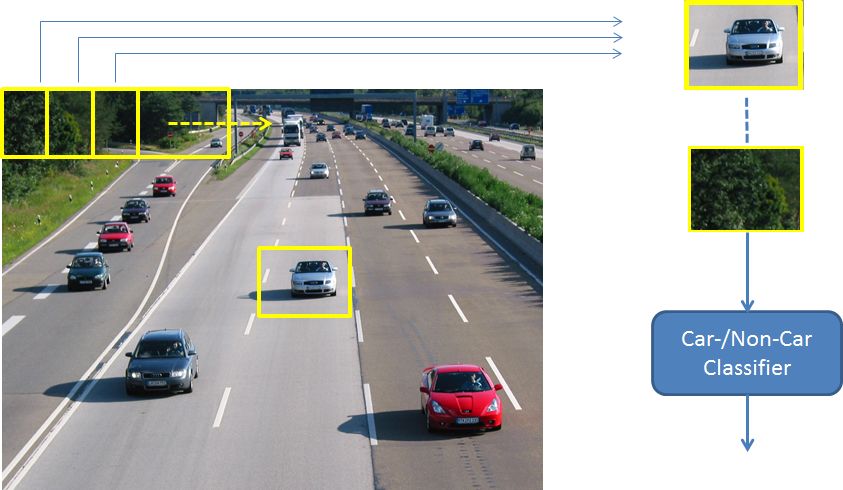
For this approach any supervised Machine-Learning algorithm can be applied, e.g. Support Vector Machines (SVM) or Mult-Layer-Perceptron. The content of a single window is either passed directly, in terms of pixel intensities, to the classifier or represented by other types of manually or automatically extracted features (see section features). The sliding window approach is computationally expensive, since windows of different sizes and aspect ratios have to be shifted in a fine-granular manner over the entire image-space
Subject of this section is another approach for object detection: Deep Neural Networks, such as R-CNN and Yolo.
Performance Measure
Intersection over Union (IoU) and mean Average Precision (mAP)
If \(A\) is the set of detected pixels and \(B\) is the set of Groundtruth-pixel, their IoU is defined to be
where \(|X|\) is the number of pixels in set \(X\). Usually two bounding boxes (pixel sets) are said to match, if their IoU is \(>0.5\). The output of the detector is correct, if
detected object = groundtruth object, and
detected bounding box and groundtruth bounding box match ( IoU is \(>0.5\))
Based on the correct and erroneous outputs the number of true positives (TP), true negatives (TN), false positives (FP), false negatives (FN) and the recall and precision can be determined. For a given class the Average Precision (AP) is related to the area under the precision-recall curve for a class:
where \(p_{interp}(r)\) is the interpolated precision at recall \(r\). The mean of these average individual-class-precisions is the mean Average Precision (mAP). More info can be obtained from PASCAL VOC Challenge
Region Proposals
Many Deep Neural Networks for Object Detection, e.g. R-CNN, require region proposals. The task of region proposal methods is to propose a list of bounding boxes within the image, which likely contain an object of interest. In order to determine these regions image-segmentation algorithms are applied, such as hierarchical clustering, mean-shift clustering or graph-based segmentation. The outputs of the applied segmentation process is often refined by methods such as selective search (see e.g. here).
R-CNN
R-CNN (Regions with CNN features) has been published 2014 in [GDDM14]. It combines Region Proposals and CNNs. As mentioned above Region Proposals are candidate boxes, which likely contain an object. R-CNN does not require a specific region proposal algorithm. However, in the experiments of [GDDM14] the authors applied Selective Search).
Inference Process
The overall R-CNN process, as depicted in the image below, consists of the following steps:
Apply Selective Search for calculating about 2000 region proposals for the given image.
Warp each region proposal to a fixed size, since the CNN requires a fixed-size input.
Pass each warped region proposal through the feature extractor-part of a CNN (modified AlexNet). The CNN-extractor provides for each region proposal a feature-vector of length 4096 to the following classifier.
Linear SVM-Classifier calculates a probability for each class. and each region proposal
Given all scored regions in an image, a greedy non-maximum suppression is applied (for each class independently) that rejects a region if it has an IoU overlap with a higher scoring selected region larger than a learned threshold.
Since the region proposals are not accurate, Bounding-Box Regression is applied to compute accurate bounding boxes. Input are coordinates of the region proposal. Output are the coordinates of the groundtruth bounding-box.

Training
R-CNN consists of 3 modells, which are trained as described below.
Training the CNN-Feature Extractor:
The CNN feature extractor is pretrained on the ILSVRC2012 imagenet data.
The CNN feature extractor is fine-tuned with the data, given in the current task in order to adapt it to the relevant domain. For this the AlexNet classifier, which is designed to distinguish 1000 classes, is replaced by a classifier, which can either distinguish 21 classes in the case of PASCAL VOC 2010 data (20 classes + background), or 201 classes in the case of ILSVRC2013.
Each batch consists of 32 positives and 96 negatives. A region proposal is labeled positive if it’s overlap with a ground-truth box is \(IoU \geq 0.5\), otherwise background.
Training the SVM:
After training and fine-tuning the CNN-feature extractor, it can be applied to calculate the 4096-dimensional feature vector for each region proposal.
The feature vectors are applied as the input of the SVM. For each class a binary linear SVM is learned.
For training SVMs only the ground-truth boxes are taken as positive examples for their respective classes and proposals with less than 0.3 IoU overlap with all instances of a class are labeled as negative for that class.
Training the Bounding-Box-Regressor:
After scoring each region proposal with a class-specific detection SVM, a new bounding box using a class-specific bounding-box regressor is predicted.
Set of \(N\) training pairs \(\{(P^i,G^i)\}\), where
specify the pixel coordinates of the center, width and height of the region proposal (P) and ground-truth (G) bounding-box, respectively.
The goal is to learn a transformation from \(P\) to \(G\) (index \(i\) is omitted ). This transformation is parametrized as follows:
where \(\hat{G}\) is the regressors prediction for \(G\). Each of the 4 function \(d_*(P)\) is modeled as a linear function
of the output \(\phi(P)\) of the last pooling layer of the CNN-extractor. The weight vectors \(w_*^T\) are learned by Ridge Regression:
where the components of the regression targets \(t\) are
R-CNN Performance and Drawbacks
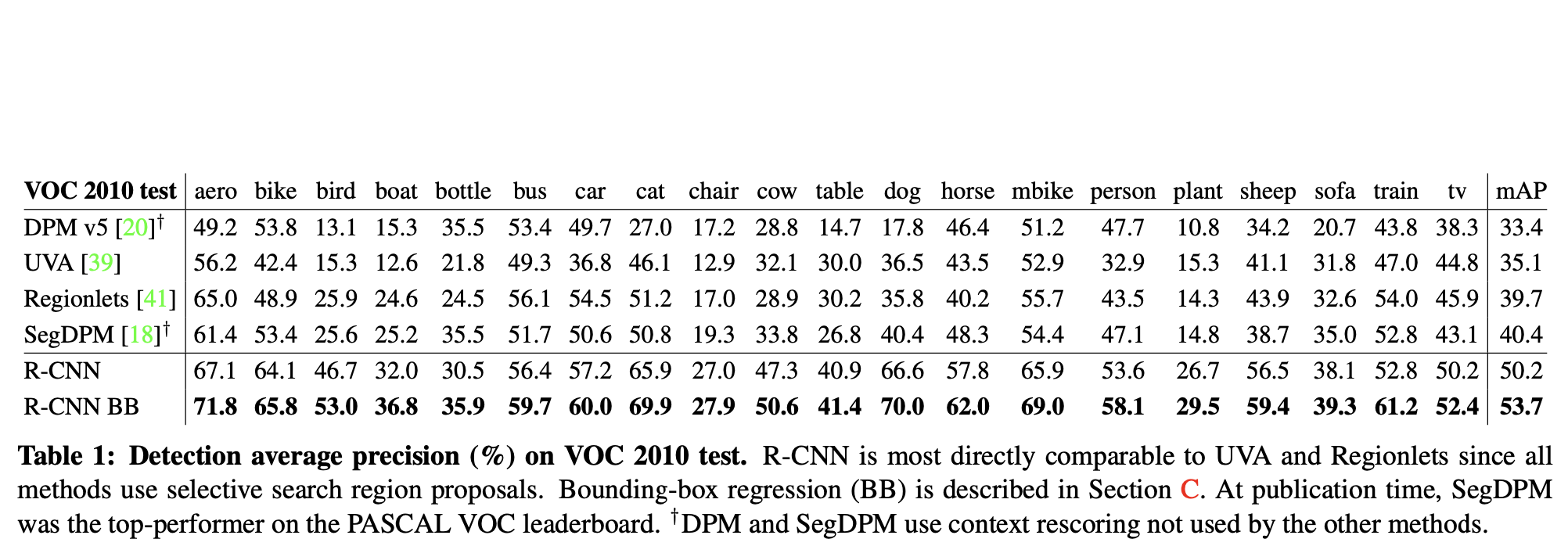
In [GDDM14] the following R-CNN performance figures were obtained:
mAP (mean Average Precision) of \(53.7\%\) on PASCAL VOC 2010- compared to \(35.1\%\) of an approach, which uses the same region proposals, but spatial pyramid matching + BoW
mAP of \(33.4\%\) on ILSVRC 2013 Detection benchmark- compared to \(24.3\%\) of the previous best result OverFeat [SEZ+]
The drawbacks of R-CNN are:
3 models must be trained
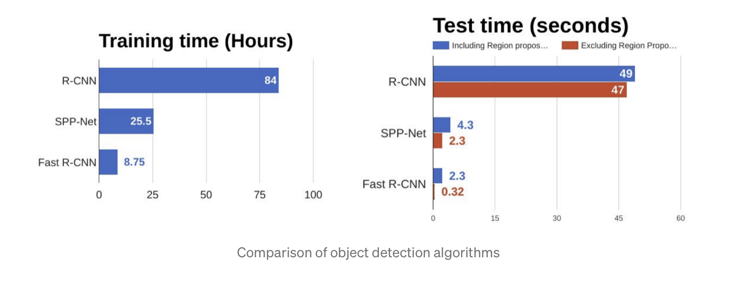
Long training time (see picture below)
About 2000 region proposals must by classified per image
Selective Search for generating the region proposals is decoupled from R-CNN. No joint-fine tuning possible
Inference time has been 47 seconds per image. Not suitable for real-time applications
In particular for small regions the warping to a fixed size CNN-input is a \alert{waste} of computational resources and yields slow detection
Spatial Pyramid Pooling (SPPnet)
Spatial Pyramid Pooling has been published 2015 in [HZRS14]. It integrates Spatial Pyramid Pooling ([LSP06]) into CNNs. SPPnet is applicable for classification and detection: In the ILSVRC 2014 challenge it achieved rank 3 and rank 2 in in the classification- and detection task respectively. Same as R-CNN, it is also based on region proposals**. However,
no warping to fixed CNN-input size is required.
it passes each image only once through conv- and pool-layers of CNN.
SPPnet is \(24-102\) times faster than R-CNN in the inference phase.
Problem of fixed size input to CNN

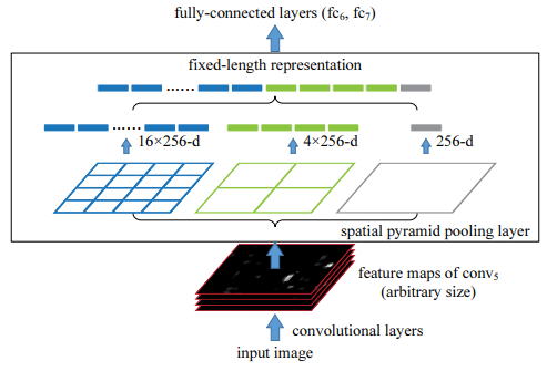
In a CNN, as depicted above, convolutional- and pooling layer can easily cope with varying input-size. However, fully connected layers require fixed-size input, because for this type varying size means varying number of weights.
SPPnet allows variable size input
Maybe, the most important contribution of SPPnet is it’s integration of a method, which is able to map an arbitray size output of the feature-extractor part to a fixed size input to the classifier part of a CNN.

Actually this mapping method to a fixed size classifier-input is the spatial pyramid pooling method as introduced long before in [LSP06]) - see also section object recognition. As sketched below, the arbitrary-sized feature maps at the output of the last convolutional layer are paritioned with an increasing granularity:
on level 0 each feature map constitutes a single region
on level 1 each feature map is partitioned into \(2 \times 2\) subregions.
on level 2 each feature map is partitioned into \(3 \times 3\) subregions.
on level 3 each feature map is partitioned into \(6 \times 6\) subregions.
Within each region max-pooling is applied to compute one value per region. The number of all regions in the entire pyramid is therefore \(1+4+9+36=50\). Since the number of all regions in the entire pyramid is independent of the size of the feature maps, the successive fully-connected layers always receive the same number of inputs. SPPnet, as defined in [HZRS14] provides 256 feature maps at the last convolution layer. Therefore the fixed-size input to the classifier has length \(50*256 = 12800\). As in R-CNN
a binary linear SVM is trained for each class (now the size of the SVM input-vectors is 12800)
a bounding box regression model is learned.
Note that with this approach, it is possible to pass the entire image only once through the CNN. Then the representation of each region proposal in the feature maps of the last conv-layer can be determined and the 256 feature maps are cropped to the size of the current region-proposal representation in this layer. Spatial pyramid max pooling, as described above, is then applied to the region proposal representation of the feature maps.
Compared to R-CNN, SPPnet achieves a slightly better mAP, whilst beeing much faster. The drawbacks of SPPnet are, that still 3 models must be trained. Moreover, the convolutional layers that precede the spatial pyramid pooling can not be fine-tuned, because the gradients of the error function can not be passed efficiently through the Spatial Pyramid Pooling). I.e. End-to-End training is not possible.
Fast R-CNN
Fast R-CNN has been published 2015 in [Gir15]. It constitutes an modification and extension of R-CNN, which is much faster in training and inference. Moreover, it achieves a higher detection quality (mAP) than R-CNN and SPPnet. It also applies region proposals (RoIs), but the image must be passed only once through the CNN. Another important improvement is that only one model must be trained using task-specific loss-functions. Fast R-CNN also requires less memory, because there is no need to store for about 2000 RoIs per image a corresponding feature vector of length 4096.
Inference Process Overview

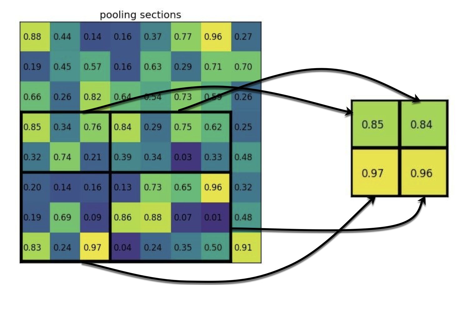
RoI Pooling Layer
A RoI of size \(h \times w\) at the last convolutional layer is partitioned into a \(H \times W\)-grid, where each region is approximately of size \(h/H \times w/W\). Typical values: \(W=H=7\). This is like level-1 partitioning in SPP. The features in each region are max-pooled, independently for each feature map.
Training
Apply pretrained CNNs
In [Gir15] three CNNs of different size are poposed. No matter which of them is applied in it’s pretrained version, three transformation steps are required to integrate it in Fast R-CNN:
the last max pooling layer is replaced by a RoI pooling layer that is configured by setting \(H\) and \(W\) to be compatible with the net’s first fully connected layer.
the network’s last fully connected layer (which was trained for 1000 objects) is replaced with the two sibling layers: a fully connected layer for \(K + 1\) categories and a category-specific bounding-box regressors.
the network is modified to take two data inputs: a list of images and a list of RoIs in those images.
Hierarchical Sampling enables Fine-Tuning
In R-CNN and SPPnet minibatches of size \(N=128\) were constructed by sampling one RoI from 128 different images. Sampling multiple RoIs from a single image was supposed to be inadequate, because RoIs from the same image are correlated, causing slow training convergence. Since at the end of the feature extractor each RoI has a large receptive field (sometimes covering the entire image), fine-tuning of the Feature Extractor would be very expensive, if each element of the batch comes from a different image. Therefore, the Feature Extractor has not been fine-tuned in R-CNN and SPPnet.
In Fast-RCNN minibatches are sampled hierarchically:
sample \(N\) images (\(N=2\)),
sample \(R/N\) RoIs from each image (\(R=128\)).
Samples from the same image share computation and memory in Forward- and Backwardpass. This yields a \(64 \times \) decrease in fine-tuning time compared to sampling \(R=128\) different images. This is why fine-tuning the feature extractor is possible in Fast R-CNN. The concern of slow convergence due to correlated samples within a minibatch has appeared to be not true in the research on Fast R-CNN.
Multi-Task Loss
Fast R-CNN has Two output-layers:
Softmax-Output with \(K+1\) neurons for class-probabilities \(p=(p_0,p_1,\ldots,p_K)\)
Bounding-Box regressors \(t^k=(t^k_x,t^k_y,t^k_w,t^k_h)\) for each of the \(K\) classes
Each training RoI is labeled with a groundtruth class \(u\) and a groundtruth bounding-box regresssion target \(v\). The multi-task loss \(L\) on each labeled RoI for jointly training classification and bounding-box regression:
where
the \([u \geq 1]\)-operator evaluates to 1 for \(u \geq 1\) and \(0\) otherwise (class-index \(u=0\) indicates no-known class).
\(L_{cls}\) is the log-loss function for true class \(u\) and \(L_{loc}\) is a \(L_1\) loss-function between the elements of the predicted- and the groundtruth bounding-box quadruple (see [Gir15]).
Faster R-CNN
Faster R-CNN has been published 2015 in [RHGS15]. In R-CNN and Fast R-CNN Selective Search) has been applied for generating the Region Proposals (RoIs). Faster R-CNN is based on R-CNN and Fast R-CNN but replaces Selective Search by a Region Proposal Network (RPN), that shares full-image convolutional features with the detection network. An RPN is a fully-convolutional network that simultaneously predicts object bounds and objectness scores at each position. RPNs are trained end-to-end to generate high- quality region proposals, which are used by Fast R-CNN for detection. With a simple alternating optimization, RPN and Fast R-CNN can be trained to share convolutional features.
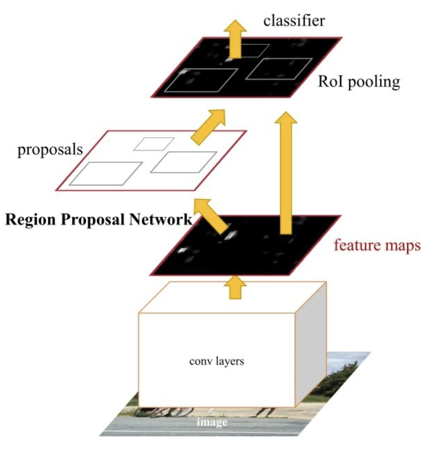
Faster-RCNNs overall process can be summarized as follows:
RPN generates region proposals, based on the last feature map of the extractor CNN
For all region proposals in the image, a fixed-length feature vector is extracted from each region using the ROI Pooling layer.
The extracted feature vectors are classified using the Fast R-CNN.
The extracted feature vectors are used to adjust the bounding-boxes
The class scores of the detected objects in addition to their bounding-boxes are returned.
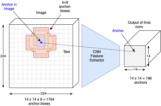
RPN
For each of the \(14 \times 14 = 196\) anchors in the input to the RPN, there exists \(k=9\) different anchor-boxes. Each anchor box is defined by its corresponding coordinates in the image \((x_c,y_c,w,h)\). To each anchor box in the training images a ground-truth-label is assigned as follows:
The label of the anchor-box is \(fg\) (foreground), if the the IoU of the anchor-box and a ground-truth bounding-box object bounding box is \(\geq 0.5\)
If the IoU is \(<0.1\) the label of the anchor-box is \(bg\) (background)
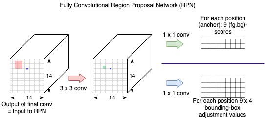
The RPN uses all the anchor-boxes selected for the minibatch of size 256 to calculate the objectness-score (foreground/background) and the corresponding classification loss using binary cross entropy. Then, it uses only those minibatch anchors marked as foreground to calculate the regression loss. For calculating the targets for the regression, the foreground anchor is compared with the closest ground-truth object in order to calculate the correct adjustment \((\Delta_{x_c},\Delta_{y_c},\Delta_{w},\Delta_{h})\). For measuring the regression error, the [RHGS15] suggests smooth L1 loss. If
\((\Delta_{x_c},\Delta_{y_c},\Delta_{w},\Delta_{h})\) is the correct adjustment
\((\delta_{x_c},\delta_{y_c},\delta_{w},\delta_{h})\) is the predicted adjustment
then the contribution of this single bounding-box to the smoothed L1-loss is defined to be
with
Smooth L1 is basically L1, but when the L1 error is small, defined by a certain \(\sigma < 1\), the error is considered almost correct and the loss diminishes at a faster rate.
Non-maximum suppression:
Since anchors usually overlap, proposals which belong to the same object may also overlap. To solve this problem Non-Maximum Suppression (NMS) is applied. NMS takes the list of proposals sorted by score and iterates over the sorted list, discarding those proposals that have an IoU larger than some predefined threshold (e.g \(IoU > 0.7\)) with a proposal that has a higher score. After applying NMS, the top \(N\) proposals, sorted by score, are kept, while the others are disregarded (\(N=2000\) in [RHGS15]).
Note that RPN can be used stand-alone, without needing the second stage model, in problems where there is only a single class of objects, the objectness probability can be used as the final class probability.
RoI-Pooling and R-CNN
Once, the region proposals are calculated by the RPN, they are passed to a RoI-Pooling such as in Fast-RCNN. The constant-length feature vector, which is provided by RoI-pooling is then past to the R-CNN, which consists of a classifier and a bounding-box regression.
Yolo
Yolo (You only look once) has been published 2015 in [RDGF15]. It is the first real-time object detector with 45 fps on Titan X GPU. A faster version even achieves 155 fps with a slightly worse accuracy. Yolo doesn’t require other modules such as region proposals. Instead it applies a single regression Pipeline, which can be learned end-to-end. YOLO sees the entire image during training and test time so it regards entire context information, which is lost in sub-window- or RoI-approaches. Hence, YOLO makes less than half the number of background errors compared to Fast R-CNN.
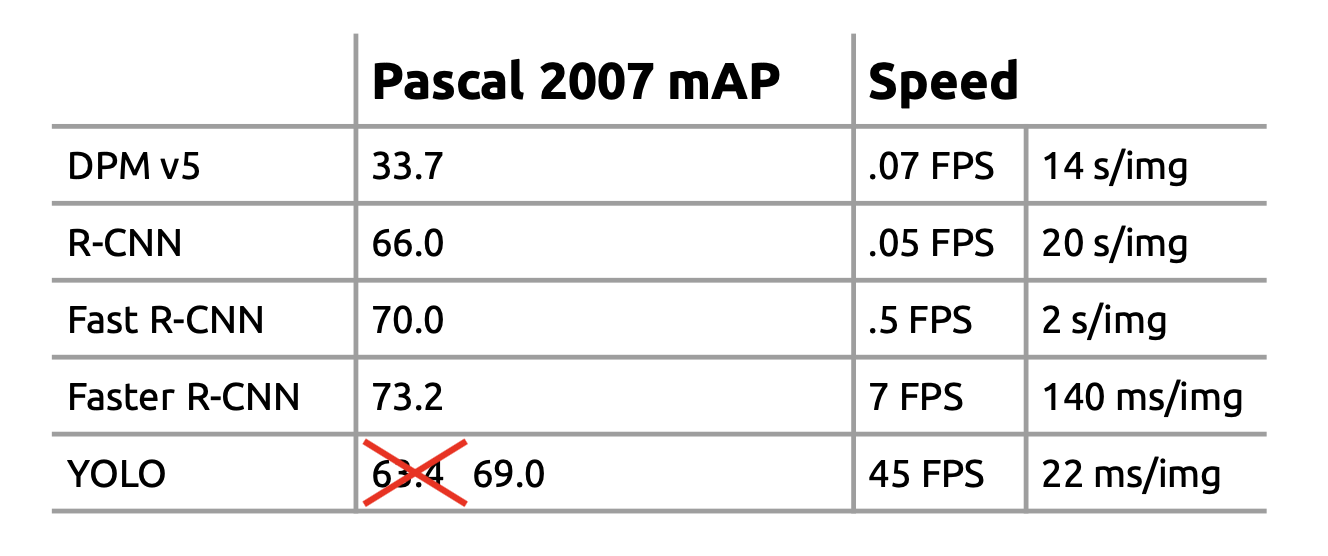
Image Source https://pjreddie.com
Concept
In Yolo the entire image is partitioned into a regular grid of \(S \times S\) cells (typical: \(S=7\)). The grid-cell which contains the center of an object is responsible to detect this object. Each grid-cell predicts \(B\) bounding boxes (typical: \(B=2\)) and confidence scores for these boxes. The confidence scores reflect
how confident the model is that the box contains an object: \(P(object)\)
how accurate the predicted box is: \(IoU(pred,truth)\)
\[ Confidence = P(object) \cdot IoU(pred,truth) \]
Each of the \(B\) bounding boxes consists of 5 predictions: \(x,y,w,h,confidence\). Each grid-cell predicts \(C\) conditional class probabilities \(P(C_j|object)\).
At test time class-specific confidence scores are calculated for all \(C\) classes.
This score reflects the probability of that class appearing in the box and how well the predicted box fits the object.
The following figure (source [RDGF15]) depicts the 49 cells, the bounding boxes and their confidence (higher confidence for thicker lines) and the most probable class for each of the 49 cells. After applying Non Maximum Suppression (NMS) the 3 bounding boxes in the image on the right remain.

Architecture
The figure below (source [RDGF15]) depicts the architecture of the first Yolo network.

The network is inspired by GoogLeNet ([SLJ+14]). Instead of the inception modules, applied in GoogLeNet, in Yolo only \((1 \times 1)\)-convolution layers (dimensionality reduction), followed by \((3 \times 3)\) convolutional layers are applied. The faster Yolo version contains only 9 instead of 24 conv-layers and less feature maps.
Yolo’s output is summarized in the image below (source https://pjreddie.com)
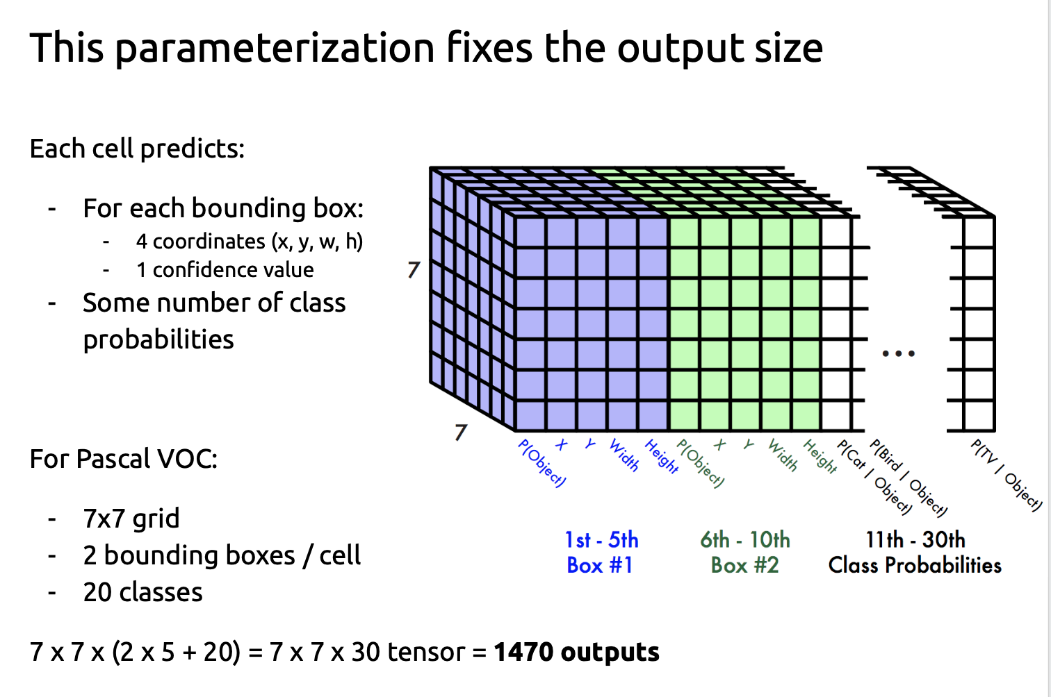
The network output is a tensor of size \( S \times S \times (5 \cdot B + C)\). With \(S=7, C=20, B=2\), this tensor contains \(49 \cdot 30\) elemenets.
Training
The convolutional-layers of the Yolo network are pretrained with the ILSVRC classification benchmark. For pretraining the first 20 convolutional layers of the architecture depicted above, followed by an average-pooling layer and a fully connected layer are applied.
After pretraining the network is adapted for object detection by:
Adding 4 additional convolutional layers and 2 fully connected layers with randomly intialized weights
Resizing the network-input layer from \((224 \times 224)\) to \((448 \times 448)\), since object detection generally requires more fine-grained features than image classification.
The final layer predicts both class probabilities and bounding box coordinates for each of the \(S^2=49\) cells. The bounding box width and height are normalized by the image width and height so that they fall between 0 and 1. The bounding box \(x\)- and \(y\)- coordinates are expressed as offsets w.r.t. a particular grid cell location so they are also bounded between 0 and 1.
During training a MSE-loss functions \(L\) is minimized, which measures the difference between the estimated output and the corresponding ground-truth. As shown in the equation for the loss-function \(L\), it weights
weights the bounding box regression
the class-specific confidence scores
the \(C\) conditional class probabilities
individually. In [RDGF15] \(\lambda_{coord}=5\) and \(\lambda_{noobj}=0.5\) are proposed. In this way the loss from predictions for boxes that don’t contain objects is decreased.
In this equation
\(\mathbb{1}_{i}^{obj}\) is 1, if a object appears in cell \(i\), otherwise 0
\(\mathbb{1}_{i,j}^{obj}\) is 1, if the j.th bounding box predictor in cell i is responsible for that prediction.
\(\mathbb{1}_{i,j}^{noobj}\) is 1, if no object is in the cell i, box j.
Moreover, in \(L\) for calulating the bounding-box width- and height- deviation the squareroot of \(w\) and \(h\) is regarded. This reflects that small deviations in large boxes matter less than in small boxes.
Drawbacks
Fully connected layer in the output implies, that all input-images have same size as training images
Although each cell can predict \(B\) bounding boxes, in the end, only the bounding box with the highest IoU is selected as the object detection output, that is, each grid can only predict one object at most. When the proportion of objects in the picture is small and each cell contains multiple objects, only one of them can be detected.
Main error of YOLO is from localization, because the ratio of bounding box is totally learned from data and YOLO makes error on the unusual ratio bounding box
Yolo v1 has been significantly improved in Yolo v2 and Yolo v3