.ipynb .pdf

Binder

Contents

Gaussian Filter and Derivatives of Gaussian

• Author: Johannes Maucher

• Last Update: 31th January 2021

Gaussian filters are frequently applied in image processing, e.g. for

• bluring

• low-pass filtering

• noise suppression

• construction of Gaussian pyramids for scaling

Moreover, derivatives of the Gaussian filter can be applied to perform noise reduction and edge detection in one step. The derivation of a Gaussian-blurred input signal is identical to filter the raw input signal with a derivative of the gaussian.

In this subsection the 1- and 2-dimensional Gaussian filter as well as their derivatives are introduced. Applications such as low-pass filtering, noise-suppression and scaling are subject of follow-up subsections.

1-dimensional Gaussian Filter

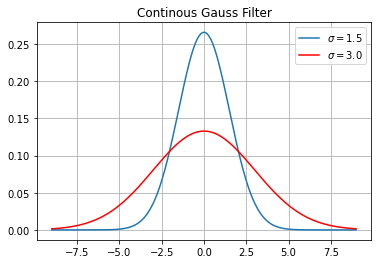
The univariate Gauss-function is defined as follows:

\[ g_{\sigma,\mu}(x) = \frac{1}{\sqrt{2 \pi} \sigma} \exp \left( - \frac{(x-\mu)^2}{2 \sigma^2}\right), \]

where \(\sigma\) is the standard deviation and \(\mu\) is the mean. In the context of filtering, the mean is always \(\mu=0\), the standard deviation \(\sigma\) is a parameter, which determines the width of the filter. In the sequel the mean is implicetly assumed to be \(\mu=0.\)

Below, two Gauss functions with different \(\sigma\) are plotted:

from matplotlib import pyplot as plt
import numpy as np
import scipy.ndimage as ndi
from matplotlib import pyplot as plt
from scipy.stats import multivariate_normal
from mpl_toolkits.mplot3d import Axes3D
from matplotlib import cm
import warnings
warnings.filterwarnings("ignore")

sigma=1.5 #standard deviation
mu=0 # mean
x=np.arange(-9,9.1,0.1)
gaussContin=gauss=1/(np.sqrt(2*np.pi)*sigma)*np.exp(-1*(x-mu)**2/(2*sigma**2))
sigma2=3
gaussContin2=gauss=1/(np.sqrt(2*np.pi)*sigma2)*np.exp(-1*(x-mu)**2/(2*sigma2**2))

plt.plot(x,gaussContin, label="$\sigma=1.5$")
plt.plot(x,gaussContin2,"r", label="$\sigma=3.0$")
plt.grid(True)
plt.title("Continous Gauss Filter")
plt.legend()
plt.show()

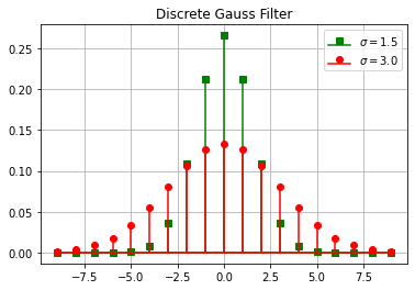
In image processing we have discrete signals (the pixels of an image) and discrete filters. For the discrete index \(u\), the discrete Gaussian filter is defined to be (for \(\mu=0\)):

\[ g_{\sigma}(u) = \frac{1}{\sqrt{2 \pi} \sigma} \exp \left( - \frac{(u)^2}{2 \sigma^2}\right), \]

For discrete Gauss-filters, u is an integer in the range

\[ u \in [-z, \ldots, z], \]

where usually \(z=\lceil 3\sigma \rceil\).

The output of the discrete Gaussian filtering, if applied to the discrete signal \(f(i)\) is than

\[ h(i) = \sum\limits_{u=-z}^{z} \frac{1}{\sqrt{2 \pi} \sigma} \exp \left( - \frac{u^2}{2 \sigma^2}\right) f(i-u) \]

Below, two discrete Gauss functions with different \(\sigma\) are plotted:

z=np.ceil(3*sigma2)
k=np.arange(-z,z+1)
gauss=1/(np.sqrt(2*np.pi)*sigma)*np.exp(-1*(k-mu)**2/(2*sigma**2))
gauss2=1/(np.sqrt(2*np.pi)*sigma2)*np.exp(-1*(k-mu)**2/(2*sigma2**2))

plt.stem(k,gauss,markerfmt="sg",linefmt="g",basefmt="g",label="$\sigma=1.5$")
plt.stem(k,gauss2,markerfmt="or",linefmt="r",basefmt="r",label="$\sigma=3.0$")
plt.grid(True)
plt.legend()
plt.title("Discrete Gauss Filter")
plt.show()

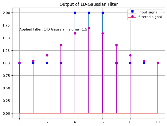
Next, the input signal x1 is filtered wit a discrete Gaussian filter with with \(\sigma=1.5\):

x1=np.array([1,1,1,1,2,2,2,1,1,1,1])
fo3=ndi.convolve1d(x1, gauss, output=np.float64, mode='nearest')

plt.figure(num=None, figsize=(8,6), dpi=80, facecolor='w', edgecolor='k')
plt.stem(x1,markerfmt="bs",linefmt='s',label="input signal")
plt.stem(fo3,markerfmt="mo",linefmt='m',label="filtered signal")
plt.title('Output of 1D-Gaussian Filter')
plt.text(0,1.65,'Applied Filter: 1-D Gaussian, sigma=1.5')
plt.grid(True)
plt.legend()
plt.show()

Instead of defining the Gauss-filter and applying the function convolve1d(), the same result can also be calculated by applying the function gaussian_filter1d() as follows:

fo3=ndi.gaussian_filter1d(x1, sigma=1.5, output=np.float64, mode='nearest')

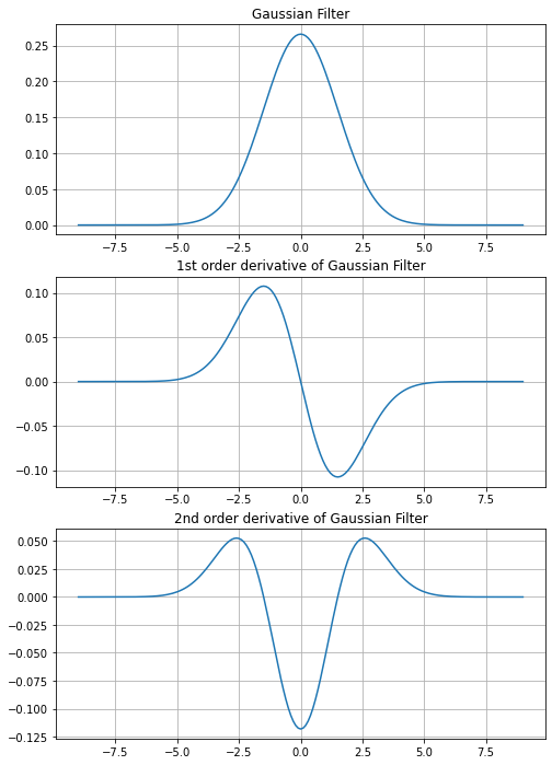
Derivatives of 1-dimensional Gaussian Filter

The 1st order derivative of the zero mean Gaussian function

\[ g_{\sigma}(x) = \frac{1}{\sqrt{2 \pi} \sigma} \exp \left( - \frac{x^2}{2 \sigma^2}\right) \]

can easily be calcultated to be

\[ g'_{\sigma}(x)=\frac{\partial g_{\sigma}(x)}{\partial x}= -\frac{x}{\sigma^2} \frac{1}{\sqrt{2 \pi} \sigma} \exp \left( - \frac{x^2}{2 \sigma^2}\right) = -\frac{x}{\sigma^2} g_{\sigma}(x), \]

And the 2nd order derivative is

\[ g''_{\sigma}(x)=\frac{\partial^2 g_{\sigma}(x)}{\partial x^2}=\left(\frac{x^2}{\sigma^4} - \frac{1}{\sigma^2} \right) \frac{1}{\sqrt{2 \pi} \sigma} \exp \left( - \frac{x^2}{2 \sigma^2}\right) = \left(\frac{x^2}{\sigma^4} - \frac{1}{\sigma^2} \right) g_{\sigma}(x). \]

Below, the gaussian function and it’s 1st and 2nd order derivative are visualized:

devxgauss=-x/sigma**2*gaussContin
devx2gauss=(x**2/sigma**4 - 1/sigma**2)*gaussContin

plt.figure(figsize=(8,12))
plt.subplot(3,1,1)
plt.grid(True)
plt.plot(x,gaussContin)
plt.title("Gaussian Filter")
plt.subplot(3,1,2)
plt.grid(True)
plt.plot(x,devxgauss)
plt.title("1st order derivative of Gaussian Filter")
plt.subplot(3,1,3)
plt.grid(True)
plt.plot(x,devx2gauss)
plt.title("2nd order derivative of Gaussian Filter")

Text(0.5, 1.0, '2nd order derivative of Gaussian Filter')

Gradient of a Signal:

In section filtering it was shown that the gradient \(\frac{\partial f}{\partial x}\) of a 1-dimensional discrete signal \(f\) can be calculated by convolving the signal with the filter \(h=(1,0,-1)\):

\[ \frac{\partial f}{\partial x}=h*f \]

By comparing the form of filter \(h\), with the first derivative of the Gaussian, it becomes obvious, that the first derivative of the Gaussian is a smoothed form of \(h\). Filtering a signal \(f\) with a Gaussian and then calculating its gradient is the same as filtering the signal \(f\) with the first order derivative of the Gaussian.

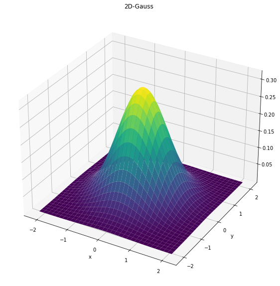
2-dimensional Gaussian Filter

A 2-dimensional continous Gaussian filter (again \(\mu=0\)) is defined as follows:

\[ G_{\sigma}(x,y) = \frac{1}{2 \pi \sigma^2} \exp \left( - \frac{x^2+y^2}{2 \sigma^2}\right) \]

The following function gauss2d(mu,sigma,order) plots either

• the 2-dimensional Gauss-function, if order=[0,0]

• the x-derivative of the 2-dimensional Gauss-function, if order=[0,1]

• the y-derivative of the 2-dimensional Gauss-function, if order=[1,0]

• the 2nd order x-derivative of the 2-dimensional Gauss-function, if order=[0,2]

• the 2nd order y-derivative of the 2-dimensional Gauss-function, if order=[2,0]

• the Laplacian of Gaussian, if order=[2,2].

def gauss2d(mu=[0,0], sigma=[1.5,1.5], order=[0,0]):
    """
    order =[0,0] plots the 2-dim Gauss function
    order =[0,1] plots the x-derivative of the 2-dim Gauss function
    order =[1,0] plots the y-derivative of the 2-dim Gauss function
    order =[0,2] plots the 2nd order x-derivative of the 2-dim Gauss function
    order =[2,0] plots the 2nd order y-derivative of the 2-dim Gauss function
    order =[2,2] plots the Laplacian of Gaussian
    """
    w, h = 100, 100

    std = [np.sqrt(sigma[0]), np.sqrt(sigma[1])]
    x = np.linspace(mu[0] - 3 * std[0], mu[0] + 3 * std[0], w)
    y = np.linspace(mu[1] - 3 * std[1], mu[1] + 3 * std[1], h)

    x, y = np.meshgrid(x, y)

    x_ = x.flatten()
    y_ = y.flatten()
    xy = np.vstack((x_, y_)).T

    normal_rv = multivariate_normal(mu, sigma)
    z = normal_rv.pdf(xy)
    z=z.reshape(w, h, order='F')
    title="2D-Gauss"
    if order == [1,0]:
        z = -x/sigma[0]**2*z.reshape(w, h, order='F')
        title="y-derivative of 2D-Gauss"
    elif order == [0,1]:
        z = -y/sigma[1]**2*z.reshape(w, h, order='F')
        title="x-derivative of 2D-Gauss"
    elif order == [0,2]:
        z = (y**2/sigma[1]**4-1/sigma[1]**2)*z.reshape(w, h, order='F')
        title="Second order x-derivative of 2D-Gauss"
    elif order == [2,0]:
        z = (x**2/sigma[1]**4-1/sigma[1]**2)*z.reshape(w, h, order='F')
        title="Second order y-derivative of 2D-Gauss"
    elif order == [2,2]:
        z = ((x**2+y**2)/sigma[1]**4-2/sigma[1]**2)*z.reshape(w, h, order='F')
        title="Second order y-derivative of 2D-Gauss" 

    fig = plt.figure(figsize=(10,10))
    ax = fig.gca(projection='3d')
    ax.plot_surface(x, y, z.T,rstride=3, cstride=3, linewidth=1, antialiased=True,
                cmap=cm.viridis)
    plt.xlabel("x")
    plt.ylabel("y")
    plt.title(title)
    plt.show()

    return z

First we plot the 2-dimensional Gauss function for \(\mu=0, \sigma=0.5\):

MU = [0,0]
SIGMA = [0.5,0.5]
z = gauss2d(MU, SIGMA, order=[0,0])

The discrete form of the Gaussian filter is

\[ G_{\sigma}(u,v) = \frac{1}{2 \pi \sigma^2} \exp \left( - \frac{u^2+v^2}{2 \sigma^2}\right), \]

where \(u\) and \(v\) are integers in the range of \([-z, \ldots, z]\), and \(z=\lceil 3\sigma \rceil\).

The convolution of a discrete 2-dimensional signal \(F\) with the 2-dimensional Gaussian filter \(G\) is then:

\[ H(i,j) = \sum\limits_{u=-k}^{k} \sum\limits_{v=-k}^{k} \frac{1}{2 \pi \sigma^2} \exp \left( - \frac{u^2+v^2}{2 \sigma^2}\right) F(i-u,j-v). \]

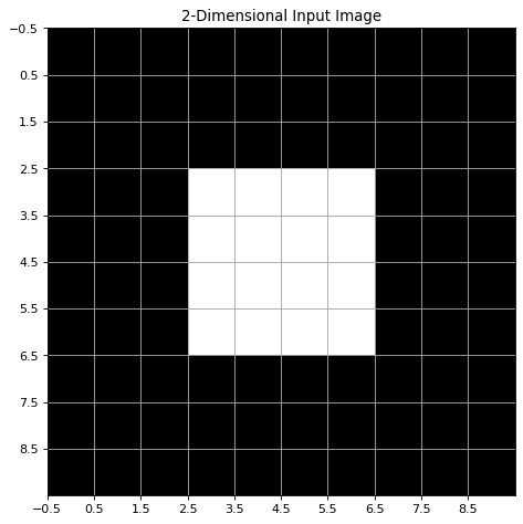
Next, 2-dimensional Gaussian filtering is demonstrated. For this we define a 2-dimensional signal \(X1\) of shape (10,10) as a numpy-array. The signal values are 1 (white) in the (4,4)-center region and 0 (black) elsewhere.

X1=np.zeros((10,10))
X1[3:7,3:7]=1

plt.figure(num=None, figsize=(14,7), dpi=80, facecolor='w', edgecolor='k')
plt.imshow(X1,cmap=plt.cm.gray,interpolation='none')
plt.xticks(np.arange(-0.5,9.5,1))
plt.yticks(np.arange(-0.5,9.5,1))
plt.grid(b=True,which='major',color='0.65')
plt.title('2-Dimensional Input Image')

Text(0.5, 1.0, '2-Dimensional Input Image')

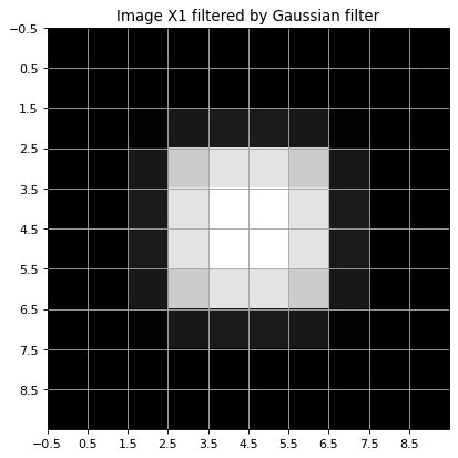
Gaussian-filtering of the image \(X1\) is performed in the following line:

fo0=ndi.gaussian_filter(X1,sigma=0.5,order=[0,0],output=np.float64, mode='nearest')

The filter output is displayed below:

plt.figure(num=None, figsize=(12,6), dpi=80, facecolor='w', edgecolor='k')
plt.imshow(fo0,cmap=plt.cm.gray,interpolation='none')
plt.xticks(np.arange(-0.5,9.5,1))
plt.yticks(np.arange(-0.5,9.5,1))
plt.grid(b=True,which='major',color='0.65')
plt.title('Image X1 filtered by Gaussian filter')

Text(0.5, 1.0, 'Image X1 filtered by Gaussian filter')

Derivatives of the 2-dimensional Gauss filter

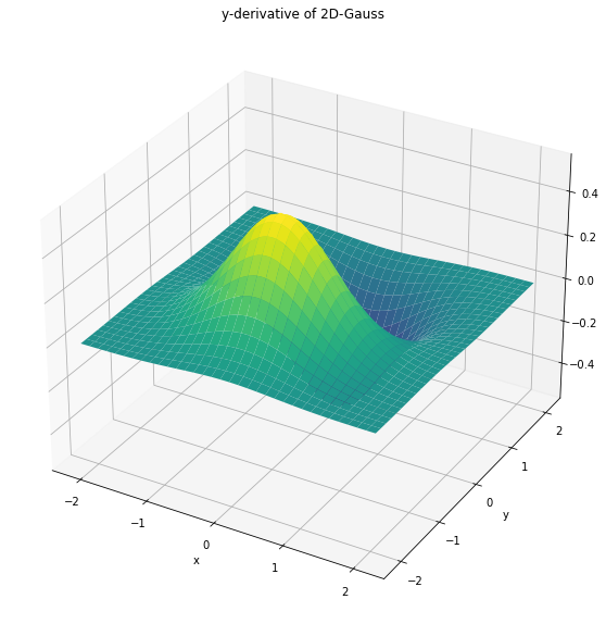
For the 2-dimensional Gaussian \(G_{\sigma}(x,y)\) the 1st order partial derivatives are

\[ \frac{\partial G_{\sigma}(x,y)}{\partial x} = -\frac{x}{\sigma^2} G_{\sigma}(x,y) \]

\[ \frac{\partial G_{\sigma}(x,y)}{\partial y} = -\frac{y}{\sigma^2} G_{\sigma}(x,y) \]

The 1st order derivatives are visualized below:

z = gauss2d(MU, SIGMA, order=[0,1])

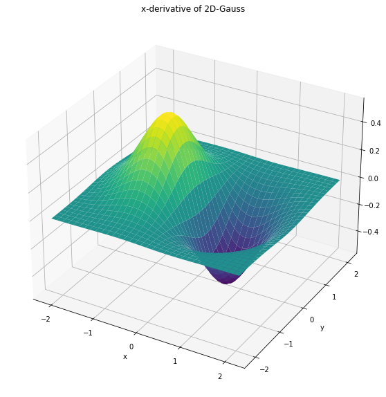
z = gauss2d(MU, SIGMA, order=[1,0])

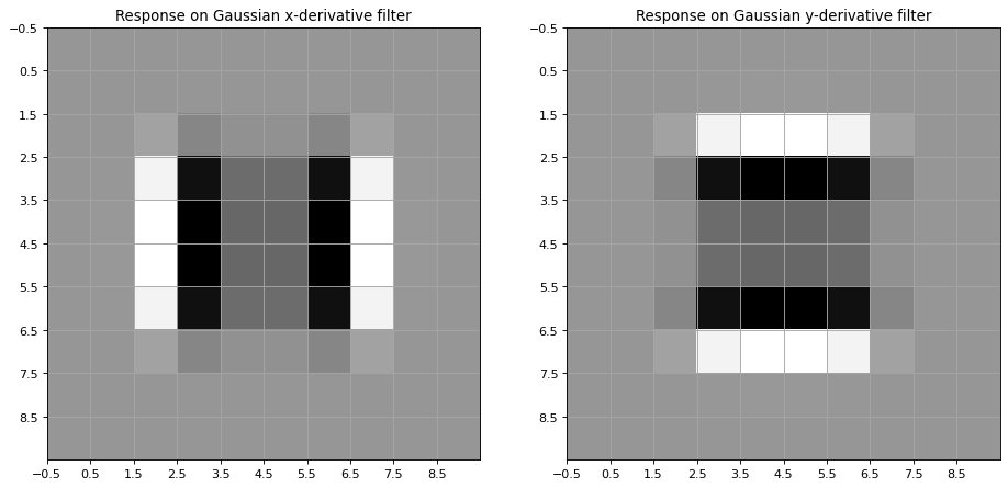
Applying the 1st order derivatives of the Gaussian to the image \(X1\) yields the output below:

fo1=ndi.gaussian_filter(X1,sigma=0.5,order=[0,1],output=np.float64, mode='nearest')
plt.figure(num=None, figsize=(14,7), dpi=80, facecolor='w', edgecolor='k')
plt.subplot(1,2,1)
plt.imshow(fo1,cmap=plt.cm.gray,interpolation='none')
plt.xticks(np.arange(-0.5,9.5,1))
plt.yticks(np.arange(-0.5,9.5,1))
plt.grid(b=True,which='major',color='0.65')
plt.title('Response on Gaussian x-derivative filter')

fo2=ndi.gaussian_filter(X1,sigma=0.5,order=[1,0],output=np.float64, mode='nearest')
plt.subplot(1,2,2)
plt.imshow(fo2,cmap=plt.cm.gray,interpolation='none')
plt.xticks(np.arange(-0.5,9.5,1))
plt.yticks(np.arange(-0.5,9.5,1))
plt.grid(b=True,which='major',color='0.65')
plt.title('Response on Gaussian y-derivative filter')
plt.show()

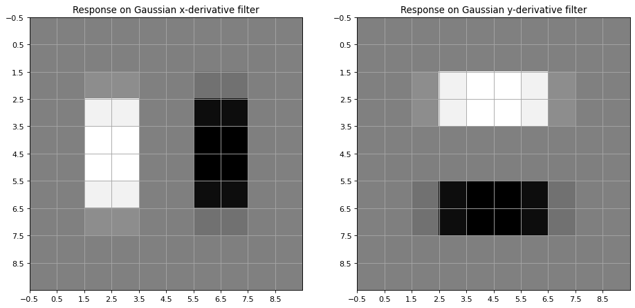
• Vertical Edges in \(F\) are extemas in

\[ \frac{\partial G}{\partial x} * F \]

• Horizontal Edges in \(F\) are extemas in

\[ \frac{\partial G}{\partial y} * F \]

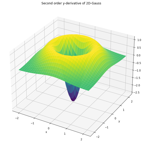
2nd order Derivatives:

Further derivation of the 1st order derivatives yields the 2nd order derivatives of the Gaussian yields:

\[ \frac{\partial^2 (G_{\sigma}(x,y))}{\partial x^2} = \left( \frac{x^2}{\sigma^4} - \frac{1}{\sigma^2} \right) G_{\sigma}(x,y) \]

(1)\[ \frac{\partial^2 (G_{\sigma}(x,y))}{\partial y^2} = \left(\frac{y^2}{\sigma^4} - \frac{1}{\sigma^2} \right) G_{\sigma}(x,y) \]

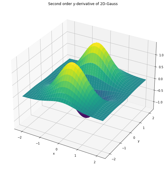
These 2nd order derivatives are visualized below:

z = gauss2d(MU, SIGMA, order=[0,2])

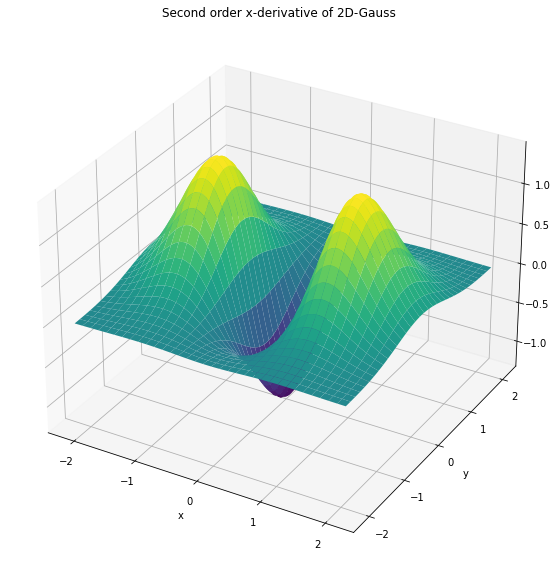
z = gauss2d(MU, SIGMA, order=[2,0])

Applying the 2nd order derivatives of the Gaussian to the image \(X1\) yields the output below:

fo3=ndi.gaussian_filter(X1,sigma=0.5,order=[0,2],output=np.float64, mode='nearest')
plt.figure(num=None, figsize=(14,7), dpi=80, facecolor='w', edgecolor='k')
plt.subplot(1,2,1)
plt.imshow(fo3,cmap=plt.cm.gray,interpolation='none')
plt.xticks(np.arange(-0.5,9.5,1))
plt.yticks(np.arange(-0.5,9.5,1))
plt.grid(b=True,which='major',color='0.65')
plt.title('Response on Gaussian x-derivative filter')

fo4=ndi.gaussian_filter(X1,sigma=0.5,order=[2,0],output=np.float64, mode='nearest')
plt.subplot(1,2,2)
plt.imshow(fo4,cmap=plt.cm.gray,interpolation='none')
plt.xticks(np.arange(-0.5,9.5,1))
plt.yticks(np.arange(-0.5,9.5,1))
plt.grid(b=True,which='major',color='0.65')
plt.title('Response on Gaussian y-derivative filter')
plt.show()

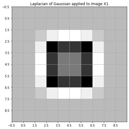
Laplacian Operator, Laplacian of Gaussian

• The Laplacian Operator \(\nabla^2 F\) is the undirected 2nd derivative of a 2-dimensional image \(F\):

\[ \nabla^2 F = \frac{\partial^2 F}{\partial x^2}+\frac{\partial^2 F}{\partial y^2} \]

• The second order derivatives of the 2-dim Gaussian filter are defined in (1)

• Smoothing an image \(F\) with a Gaussian and then taking its Laplacian operator is equivalent to convolving the image \(F\) with the Laplacian of Gaussian (LoG) Filter:

\[ \nabla^2 G_{\sigma}(x,y)=\left(\frac{x^2+y^2}{\sigma^4} - \frac{2}{\sigma^2}\right) G_{\sigma}(x,y) \]

z = gauss2d(MU, SIGMA, order=[2,2])

• Edges in \(F\) are zero crossings of the Laplacian operator applied to \(F\)

The Laplacian of Gaussian is a robust method to detect edges in images. Below the scipy-method gaussian_laplace() is applied to calculate the Laplacian of Gaussians of the image \(X1\). The output is visualized. Moreover, the values of the output are ploted. As can be seen the zero-crossings (same as switch of sign) are actually at the edges of the input image.

fo5=ndi.gaussian_laplace(X1,sigma=0.5,output=np.float64, mode='nearest')

plt.figure(figsize=(7,7))
plt.imshow(fo5,cmap=plt.cm.gray,interpolation='none')
plt.xticks(np.arange(-0.5,9.5,1))
plt.yticks(np.arange(-0.5,9.5,1))
plt.grid(b=True,which='major',color='0.65')
plt.title('Laplacian of Gaussian applied to Image X1')
plt.show()

Values of output:

np.set_printoptions(precision=1,suppress=True)

fo5

array([[ 0. ,  0. ,  0. ,  0. ,  0. ,  0. ,  0. ,  0. ,  0. ,  0. ],
       [ 0. ,  0. ,  0. ,  0. ,  0. ,  0. ,  0. ,  0. ,  0. ,  0. ],
       [ 0. ,  0. ,  0.3,  1. ,  1.2,  1.2,  1. ,  0.3,  0. ,  0. ],
       [ 0. ,  0. ,  1. , -3.3, -2.4, -2.4, -3.3,  1. ,  0. ,  0. ],
       [ 0. ,  0. ,  1.2, -2.4, -1.2, -1.2, -2.4,  1.2,  0. ,  0. ],
       [ 0. ,  0. ,  1.2, -2.4, -1.2, -1.2, -2.4,  1.2,  0. ,  0. ],
       [ 0. ,  0. ,  1. , -3.3, -2.4, -2.4, -3.3,  1. ,  0. ,  0. ],
       [ 0. ,  0. ,  0.3,  1. ,  1.2,  1.2,  1. ,  0.3,  0. ,  0. ],
       [ 0. ,  0. ,  0. ,  0. ,  0. ,  0. ,  0. ,  0. ,  0. ,  0. ],
       [ 0. ,  0. ,  0. ,  0. ,  0. ,  0. ,  0. ,  0. ,  0. ,  0. ]])

Basic Filter Operations Rectangular- and Gaussian Low Pass Filtering