
Local Image Features
In contrast to global features, local features describe not the entire image, but only a local region within the image. As depicted in the figure below, for each image usually a large set of local descriptors is obtained. Actually in the image below, not the local descriptors itself, but the keypoints are shown by blue markers. Usually one first finds keypoints, then the area around each keypoint is described by a local descriptor, which is usually a numeric vector.
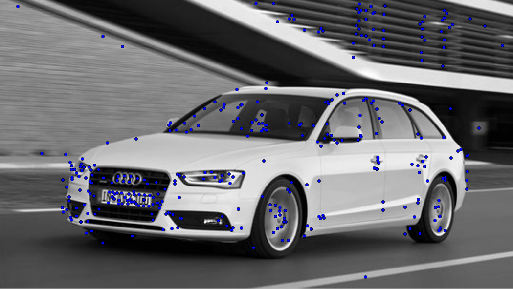
In most applications, local features provide much more robustness than global features. Depending on the specific type of local feature, they can be robust w.r.t. rotation, translation, viewpoint, scale, ligthing partial deformation and partial occlusion.
In [GL11] local features are defined as follows:
Local Features
The purpose of local invariant features is to provide a representation that allows to efficiently match local structures between images. That is, we want to obtain a sparse set of local measurements that capture the essence of the underlying input images and that encode their interesting structure.
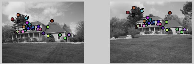
Image Source: http://cs.brown.edu/courses/cs143/results/proj2/sphene/
General Requirements and Categorization
According to [TM07] local features in general shall have the following characteristics:
Repeatability: Given two images of the same object, taken under different viewing conditions, a high percentage of the features detected on the object part visible in both images should be found in both images.
Distinctiveness/informativeness: The intensity patterns underlying the detected features should show a lot of variation, such that features can be distinguished and matched. By looking through a small window it must be easy to localize the point. Shifting the window in any direction should give a large change in pixel intensities, gradients, …
Locality: The features should be local, so as to reduce the probability of occlusion and to allow simple model approximations of the geometric and photometric deformations between two images taken under different viewing conditions.
Quantity: The number of detected features should be sufficiently large, such that a reasonable number of features are detected even on small objects. However, the optimal number of features depends on the application. Ideally, the number of detected features should be adaptable over a large range by a simple and intuitive threshold. The density of features should reflect the information content of the image to provide a compact image representation.
Accuracy: The detected features should be accurately localized, both in image location, as with respect to scale and possibly shape.
Efficiency: Preferably, the detection of features in a new image should allow for time-critical applications.
Applications, which integrate local features can be categorized in an abstract level as follows ([TM07]):
Interest in a specific type of local feature that has a clear semantic interpretation in the context of a given application. E.g. in aerial images edges indicate roads.
Interest in local features since they provide a limited set of well localized and individually identifiable anchor points (e.g. for tracking applications or image stichting).
Use set of local features as a robust image representation. Allows for object- or scene recognition without image segmentation.
In the second and third category the semantics of the local feature are not relevant.
An example for the second category is image stitching:
First keypoints are detected in both images. Then pairs of corresponding keypoints must be found. The locations of the matching pairs are then used to align the images.


An example for the third category is object identification: First local features from both images are extracted independently. Then candidate matching pairs of descriptors must be determined. From the location of the matching pairs the most probable geometric configuration can be determined and verified.

Harris-Förstner Corner Detection
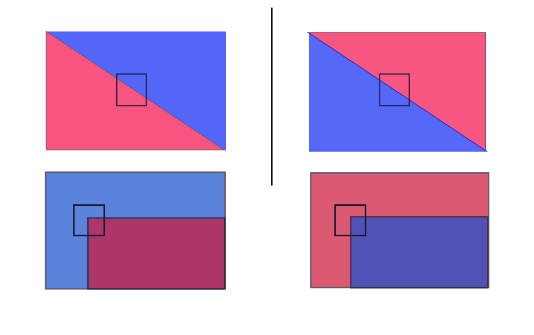
As stated above an important criteria for good keypoints is:
Shifting the small window in any direction should give a large change in gradients.
According to [HS88] the change of gradients in the neighborhood of a pixel can be determined as follows:
Calculate the gradient at position \(\mathbf{x}\):
(9)¶\[\begin{split} \nabla I(\mathbf{x}) = \left( \begin{array}{c} \frac{\partial I(\mathbf{x})}{\partial x} \\ \frac{\partial I(\mathbf{x})}{\partial y} \end{array} \right) = \left( \begin{array}{c} I_x(\mathbf{x}) \\ I_y(\mathbf{x}) \end{array} \right) \end{split}\]The gradients are calculated by applying the 1st order derivative of a Gaussian (see chapter Image Processing).
At each position \(\mathbf{x}\) calculate the matrix
\[ \begin{align}\begin{aligned}\begin{split} M_I(\mathbf{x}) = \nabla I(\mathbf{x}) \nabla I^T(\mathbf{x}) = \left( \begin{array}{c} I_x(\mathbf{x}) \\ I_y(\mathbf{x}) \end{array} \right) \left( I_x(\mathbf{x}) \quad I_y(\mathbf{x}) \right)\end{split}\\\begin{split} = \left( \begin{array}{cc} I_x^2(\mathbf{x}) & I_x I_y(\mathbf{x}) \\ I_x I_y(\mathbf{x}) & I_y^2(\mathbf{x}) \end{array} \right) \end{split}\end{aligned}\end{align} \]Average matrices \(M_I(\mathbf{x})\) over a region by convolution with a Gaussian \(G_{\sigma}\):
(10)¶\[ C(\mathbf{x},\sigma)=G_{\sigma}(\mathbf{x}) * M_I(\mathbf{x}) \]Depending on the local image properties in the region defined by the width of \(G_{\sigma}\) the Eigenvalues \(\lambda_1\) and \(\lambda_2\) of matrix \(C(\mathbf{x},\sigma)\) vary as follows:
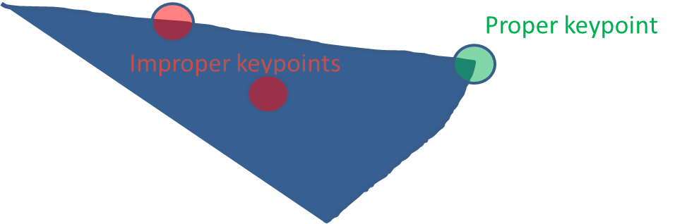
If both Eigenvalues are large, then there is a corner around \(\mathbf{x}\)
If one Eigenvalue is large, and the other is \(\approx 0\), then there is an edge around \(\mathbf{x}\).
If both Eigenvalues are \(\approx 0\), then there is no variation in the region around \(\mathbf{x}\).
Note that \(C(\mathbf{x},\sigma)\) and it’s Eigenvalues must be calculated at each position \(\mathbf{x}\) and the calculation of Eigenvalues is costly. However, there is a trick to perform the differentiation, mentioned in item 4 above, without calculating the Eigenvalues. For this let \(\alpha\) be the Eigenvalue with the larger and \(\beta\) be the Eigenvalue with the smaller magnitude. Morevoer,
is the ratio of these Eigenvalues.
Calculate trace and determinant of \(C(\mathbf{x},\sigma)\)
\[ Tr(\mathbf{C(\mathbf{x},\sigma)}) = \alpha + \beta \]\[ Det(\mathbf{C(\mathbf{x},\sigma)}) = \alpha \beta \]Then
(11)¶\[ \frac{Tr(\mathbf{C(\mathbf{x},\sigma)})^2}{Det(\mathbf{C(\mathbf{x},\sigma)})} = \frac{(\alpha + \beta)^2}{\alpha \beta} = \frac{(r \beta + \beta)^2}{r\beta^2}=\frac{(r+1)^2}{r} \]depends only on the ratio \(r\) of eigenvalues.
Corners are at the points where this value is small.
In order to check if the value in equation (11) is small one can equivalently check if
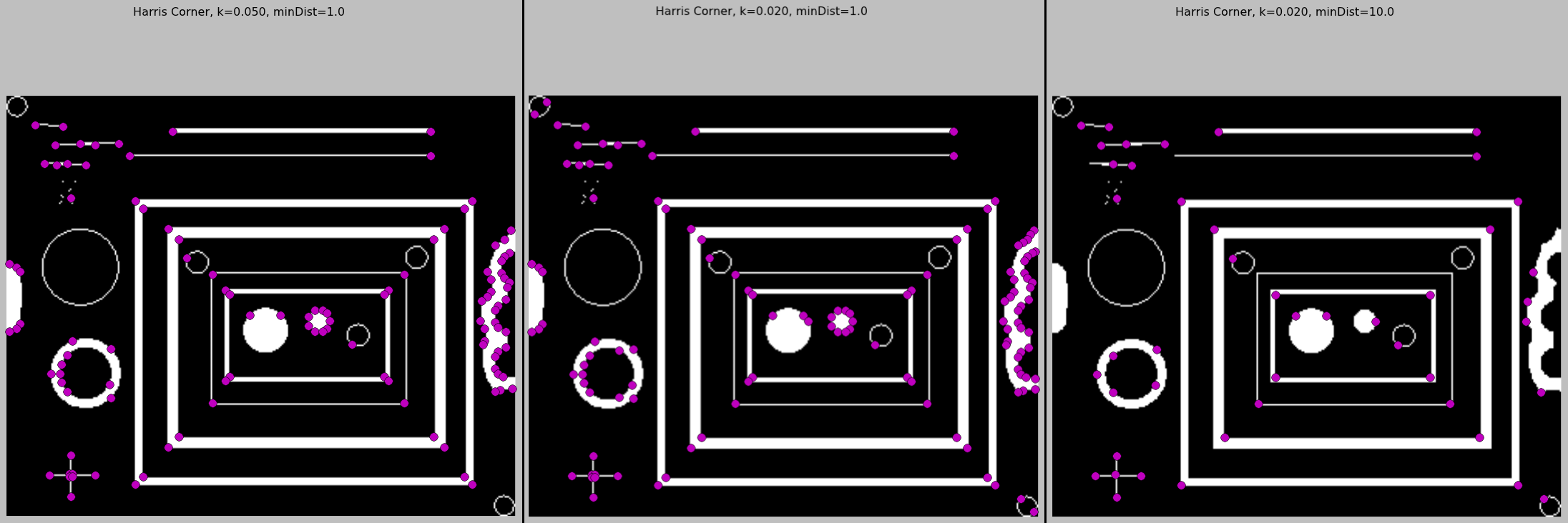
Concerning the parameters in in the described process:
\(\kappa\) is in the range \([0.04,\ldots 0.15]\). Smaller \(\kappa\) yields more detected corners.
If the standard deviation of the Gaussian filter, used to calculate the derivatives in equation (9) is \(\sigma_d\), then the standard deviation \(\sigma\) of the Gaussian, used in equation (10), should be \(\sigma \approx 2\sigma_d\). Typical value: \(\sigma=1.0\) i.e. \(\sigma_d \approx 0.5\).
In implementations, e.g. Scikits Image, usually one function calculates for all pixels the value, given in the left hand side of unequation (12) and a second function applies the threshold \(T\) (default value 0) and a minimum distance \(D_{min}\) to the result of the first function. Detected corners are then separated by at least \(D_{min}\) pixels. The influence of varying parameters \(\kappa\) and \(D_{min}\) is demonstrated in the picture below):
In section harrisCornerDetection an implementation of Harris-Corner detection is demonstrated.
Even though Harris-Förstner corner detection is translation- and rotation-invariant, one major drawback is that it is not scale-invariant. As depicted in the picture below, the approach can find corners if the object is given in a small scale. However, if the object is represented in a higher scale there may be now detected corners in the same object-area.

An approach for scale-invariant features is described in the following subsection.
Scale Invariant Feature Transform (SIFT)
Scale Invariant Feature Transform (SIFT) is an algorithm to detect and describe local features in images. It has been introduced in [Low04]. SIFT features are invariant w.r.t. translation, rotation, scale and quite robust w.r.t. illumination, 3D viewpoint, additional noise and partial occlusion. The SIFT process consists of the following steps:
Phase 1: Scale space extrema detection
Search potential keypoints by determining extremas in scale space.
Phase 2: Keypoint localization and filtering
Keypoint localization and filtering
Phase 3: Orientation Assignment
One or more orientations are assigned to each keypoint location.
Phase 4: Keypoint descriptor
Local image gradients are measured at the selected scale in the region around each keypoint
Scale space extrema detection
Scale Space of input image \(I(x,y)\):
\[ L(x,y,\sigma)=G(x,y,\sigma) * I(x,y) \]Variable Scale Gaussian:
\[ G(x,y,\sigma)= \frac{1}{2\pi\sigma^2}e^{-\dfrac{x^2+y^2}{2\sigma^2}} \]Difference of Gaussian (DoG):
DoG has already been introduced in Gaussian and Difference of Gaussian Pyramid. It is
efficient to compute - the smoothed images L must be computed in any case for the scale space feature description
a close approximation to the scale-normalized Laplacian of Gaussian, whose extremas produce the most stable image features ([Low04])
Scale space and the DOGs are visualized in the image below (Source: [Low04]). An octave means doubling of \(\sigma\). The scale space resolution is \(k=2^{1/s}\), where \(s\) is the number of scales per octave. After each octave the image is subsampled by a factor of \(2\). For each octave \(s+3\) blurred images are required to determine scale space extrema (see next slide). A typical resolution is \(s=3\).

The scale space of a concrete image is depicted below:

As shown in the image below, in the DoG each pixel is compared with its 26 neighbour pixels at the current and adjacent scales. The Pixel is selected as a keypoint candidate, if it is larger than all of the neighbours (maxima) or smaller than all of them (minima).

Keypoint localization and filtering
The set of keypoint candidates is refined as follows:
Determine exact position of local extremas on sub-pixel resolution
Select within the set of candidate keypoints only the stable and distinctive ones. Candidate keypoints with low contrast are not stable, because they are sensitive to noise. Moreover, candidate keypoints on edges are not distinctive.
Exact Keypoint Localization
In the previous step candidate keypoints have been localized on pixel level. Note that particularly for candidates on a high level of the DoG (where images are at a low-resolution) a localization on pixel-level is quite inaccurate. Therefore, the keypoint-localization must be improved to sub-pixel level. In general there exist two possibilities to estimate sub-pixel information. The first is interpolation, the second is by Taylor-series expansion.
The idea of interpolation is depicted in the image below:
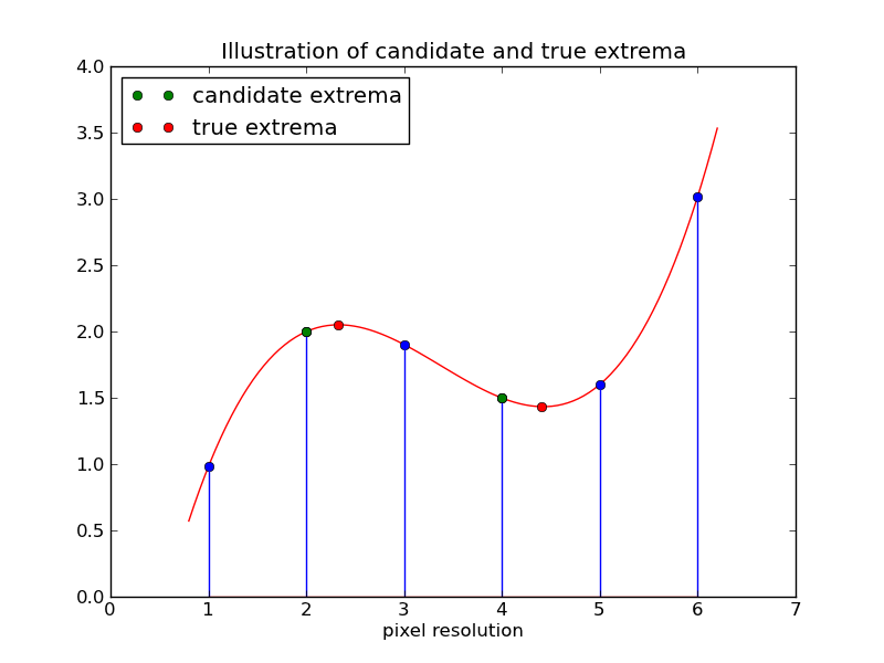
However, in SIFT Taylor-series expansion is applied for refining keypoint localization.
Taylor expansion of \(D(x,y,\sigma)\) up to quadratic forms around the sample point (keypoint candidate) is defined as follows:
Here \(\mathbf{x}=(x,y,\sigma)^T\) is the offset from the candidate keypoint and the first and second derivation are:
The derivatives of \(D\) are approximated by calculating differences in the \((3x3)\)-neighbourhood. The true location \(\hat{\mathbf{x}}\) of the keypoint is determined by taking the derivative of (13) and setting it to zero:
If the offset \(\hat{\mathbf{x}}\) is \(>0.5\) in any dimension, then the extremum lies closer to different sample point and new interpolation starts centered at this new point.
Reject Low Contrast Candidates
Pixels of low contrast can be determined by low DoG values. If the image values are normalized to the range \(\left[0,1\right]\), candidates with
are rejected as low contrast points.
Reject Candidates on Edges
DoG values can not uniquely locate points on edges (since all points on the edge have similar DoG values), but in corners. Since edges constitute extremas in the DoG and are therefore selected as candidates in the first step, they must be filtered out now. The idea of the edge-rejection approach in SIFT is based on the fact, that at edges the DoG function will have a large prinicpal curvature across the edge, but a relatively small curvature in the orthogonal direction (along the edge). Keypoint candidates, which fulfill this criteria are rejected.
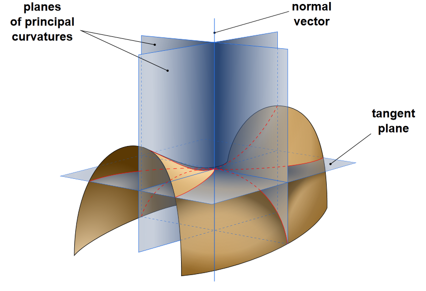
The curvature-test is implemented as follows:
The two eigenvalues of the 2D Hessian
are proportional to the principal curvatures.
Denote:
\(\alpha\): eigenvalue with larger magnitude
\(\beta\): eigenvalue with smaller magnitude
A large ratio
indicates a large curvature in one direction and a small in the perpendicular direction \(\Rightarrow\) Edge.
Calculate trace and determinant of \(\mathbf{H}\)
then
depends only on the ratio \(r\) of eigenvalues.
In [Low04] candidates with \(r>10\) are rejected as edges.
The following picture displays the contrast-dependent and the curvature-dependent candidate rejection.

Orientation Assignment
This step is required in order to provide an image-descriptor, which is invariant to image-rotation. The idea is to calculate for each keypoint, remained from the previous steps, an orientation from it’s local image properties.
Create Orientation Histogram
From the scale of the keypoint, select the Gaussian smoothed image, \(L\), with the closest scale.
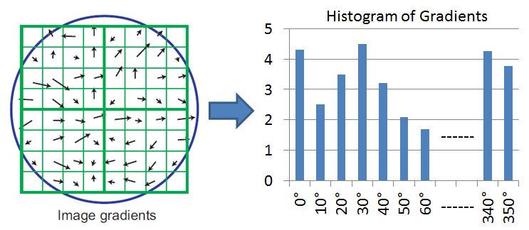
For each image sample, \(L(x,y)\) at the selected scale compute gradient magnitude:
\[ m(x,y)=\sqrt{(L(x+1,y)-L(x-1,y))^2+(L(x,y+1)-L(x,y-1))^2} \]and gradient orientation
\[ \theta(x,y) = arctan \frac{L(x,y+1)-L(x,y-1)}{L(x+1,y)-L(x-1,y)} \]Calculate a 36 bin gradient histogram (\( 1 bin \triangleq 10°\)) from the gradients of the samples in the local neighbourhood of the keypoint. The contribution of each gradient to the histogram is the product of
its magnitude \(m(x,y)\)
and the value \(g(x',y')\), where \(g(x',y')\) is a circular Gaussian window, centered at the keypoint \((x,y)\). The standard deviation \(\sigma\) is \(1.5\) times the scale of the keypoint.
Assign Orientations to Keypoints
For each histogram the orientations with the
the peak value
values \(>80\%\) of the histogram’s peak
constitute keypoint orientations. Thus for a given keypoint location, \(>1\) keypoints can be generated. In the average \(15\%\) of all keypoints have multiple orientations. To provide better accuracy of the keypoint orientations quadratic interpolation w.r.t. the \(3\) closest histogram values is applied.
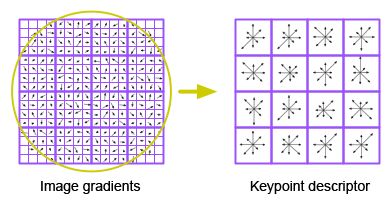
Keypoint descriptor
For each of the remaining keypoints a descriptor, i.e. a numeric vector of predefined length, is calculated as follows:
Determine gradient magnitude and orientations at all points around the keypoint as described above. In the pictures below two options for the size of the keypoint neighbourhood are shown. In the topmost image the \(8x8\) pixels around the keypoint constitute the neighbourhood. In the second image the neighbourhood consists of the \(16x16\) pixels around the keypoint. This neighbourhood-size is a parameter, which can be configured. As shown below a large neighbourhood-yields a longer feature-descriptor.
In order to achieve orientation invariance, the coordinates of the descriptor and the gradient orientations are rotated relative to the keypoint orientation.
A Gaussian weighting function with \(\sigma\) equal to one half the width of the descriptor window is used to assign a weight to the magnitude of each sample point. Thus the influence of sample points at the window boundary is reduced and the keypoint descriptor is less sensitive to small shifts of the window.
For each of the \((4x4)\)-subregions a single histogram is created.
Each histogram has 8 bins (directions).
For a neighbourhood-size of \((8x8)\) (topmost image below), there are \(4\) subregions. Each subregion is described by a histogram of 8 bins and the final keypoint descriptor is a vector of \(4 \cdot 8 = 32\) elements. For a neighbourhood-size of \((16x16)\) (second image) there are \(16\) subregions. Each subregion is described by a histogram of 8 bins and the final keypoint descriptor is a vector of \(16 \cdot 8 = 128\) elements.

Note that the descriptor may change abruptly if a sample shifts smoothly from
one histogram to another
one orientation bin to another
In order to avoid such abrupt changes, trilinear interpolation, which distributes the value of each gradient sample into adjacent histogram bins, is usually applied.
SIFT descriptors are not only translation-, rotation- and scale-invariant. They are also robust w.r.t. illumination (contrast and brightness) changes. A contrast change is basically a multiplication of all pixel-values with a constant factor. Then the gradients are multiplied by the same constant, but this constant is cancelled out in the case that the histograms are normalized to unit length. A brightness change is an addition of a constant to all pixel values. An additonal constant does not have any impact on the gradients, therefore the descriptor is also invariant w.r.t. a homogenous brightness variation.