
Convolutional Neural Networks for Object Recognition
ImageNet Contest
The ImageNet Large Scale Visual Recognition Challenge (ILSVRC) evaluates algorithms for object detection and image classification at large scale. It contains
Detection challenge on fully labeled data for 200 categories of objects
Image classification challenge with 1000 categories
Image classification plus object localization challenge with 1000 categories
The Training data, provided for the challenge is a subset of ImageNet data. ImageNet is an image database organized according to the WordNet hierarchy, in which each node of the hierarchy is depicted by hundreds and thousands of images. (15 million images in 22000 categories).

Detection Challenge
In the detection challenge 200 object categories must be distinguished. Training data consists of 456567 images with 478807 objects. For validation 20121 images with 55502 objects from flickr and other search engines are provided. The test-dataset consists of 40152 images from flickr and other search engines. The average image resolution in validation data is: \(482 \times 415\) pixels. For each image, the algorithms must produce a set of annotations \((c_i,b_i,s_i)\) of class labels \(c_i\), bounding boxes \(b_i\) and confidence scores \(s_i\).

Classification Challenge
In the classification challenge 1000 object categories are distinguished Training data consists of 1.2 Million images from ImageNet. For validation 50 000 images from flickr and other search engines are provided. The test-dataset consists of 100 000 images from flickr and other search engines. For each image the algorithms must produce \(5\) class labels \(c_i, \, i \in \lbrace1,\ldots,5\rbrace\) in decreasing order of confidence and 5 bounding boxes \(b_i, \, i \in \lbrace1,\ldots,5\rbrace\), one for each class label. The Top-5 error rate is the fraction of test images for which the correct label is not among the five labels considered most probable by the model.
In the localisation-task object-category and bounding boxes must match. Bounding boxes are defined to match, if they have an overlap (Intersection over Union) of \(>50\%\).
AlexNet
AlexNet is considered to be an important milestone in Deeplearning. This CNN has been introduced in [KSH] and won the ILSVRC 2012 classification- and localisation task. It achieved a top-5 classification error of \(15.4\%\) (next best achieved \(26.2\%\)!).
The key elements of AlexNet are:
ReLu activations decrease training time
Local Response Normalisation (LRN) in order to limit the outputs of the Relu activations
Overlapped Pooling regions
For reducing overfitting Data augmentation and Dropout are applied.
Data Augmentation: For training not only the \(224 \times 224\) crop at the center, but several crops within the \(256 \times 256\) image are extracted. Moreover, also their horizontal flips are applied and the intensities of the RGB channels have been altered to provide more robustness w.r.t. color changes. The augmented training dataset consisted of 15 million annotated images
Dropout is applied in the first 2 fully-connected-layers
Training duration 6 days on two parallel GTX 580 3GB GPUs


At the input AlexNet requires images of size \(256 \times 256\). Since ImageNet consists of variable-resolution images, in the preprocessing the rectangular images are first rescaled such that shorter side is of length \(256\). Then the central \(224 \times 224\) patch is cropped from the resulting image. In addition to this scaling, the only preprocessing routine is subtraction of the mean value over the training set from each pixel.
In the test-phase from each test - image 10 versions were created:
the four \(224 \times 224\) corner crops and the center crop
from each of the 5 crops the horizontal flip
For the 10 versions the corresponding output of the softmax-layer is calculated and the class which yields highest average output over the 10 versions is selected.

VGG Net
In [KS14] the Visual Geometry Group of the Universitiy of Oxford introduced the VGG Net. The main goal of the researches was to investigate the influence of depth in CNNs. VGG Net won the ILSVRC 2014 localisation-challenge and became \(2nd\) in the classification task.
The architecture of VGG-13 (13 learnable layers) is shown below:

All VGG versions are summarized in this table:

The number of parameters in these versions are millions:
A, A-LRN: 133 millions
B: 133 millions
C: 134 millions
D: 138 millions
E: 144 millions
As can be seen only version A-LRN contains Local Response Normalisation. In the experiments this version did not perform better than the version A without LRN.
The key facts of the VGG-architecture are:
\(224 \times 224 \) RGB images at the input
Preprocessing: Subtract mean-RGB image computed on trainings set.
Small receptive fields of \(3 \times 3\) in filters, particularly in the first conv-layers.
Stride: \(1\)
Padding: \(1\) for \(3 \times 3\)-filters
\(2 \times 2\)-Max-Pooling with stride 2
ReLu activation in all hidden layers
No Normalization
Feature Maps: 64 in the first layer and increasing by a factor of 2 after each pooling layer.
All VGG versions apply only filters of size \(3 \times 3\). The apparent drawback of small filters may be that only small features in the input can be extracted. This assumption is not valid, if the local receptive fields of a sequence of layers is considered: A stack of two conv-layers with \(3 \times 3\) receptive field has an effective receptive field of \(5 \times 5\) and a stack of three conv-layers with \(3 \times 3\) receptive field has an effective receptive field of \(7 \times 7\). The advantages of a stack of layers with smaller filters are:
Stacked version has more ReLu-nonlinearities, which enables more discriminative decision function
Stacked version has less parameters:
\(3 \cdot 3^2C^2 = 27C^2\) for a 3-layer stack of \((3 \times 3)\)-filters, versus …
\(7^2C^2=49C^2\) for a single layer with \((7 \times 7)\)-filters
where \(C\) is the number of channels (feature maps in the layer). Less parameters impose better generalisation.
The VGG experiments prove that it is better to apply more layers with small filters than less layers with larger filters.
The images passed to the input of VGG are of size \(224 \times 224\). In the training phase this input is cropped from a training image, which is isotropically rescaled. The smallest side of the rescaled training image is called training scale \(S\). There exist two options for setting \(S\):
Use constant \(S\) (single-scale training}, e.g. \(S=256\) or \(S=384\).
multi-scale training: randomly sample \(S\) from a range e.g. \([256,512]\).
Results of single- and multiscale-testing are listed in the tables below:


GoogLeNet (Inception)
GoogLeNet, a 22-layer network based on the concept of inception, has been introduced in [SLJ+14]. It won the ILSVRC 2014 image classification challenge and attained a significant better error rate than AlexNet and VGG-19, while requiring 10 times less parameters than AlexNet.
The research goal of the authors was simply to find a neural network architecture, which attains higher accuracy with an as small as possible number of learnable parameters. The obvious way to improve the accuracy is to just stack more and more layers on top of each other or to increase the number of neurons (number of feature maps) in a layer. However, this strategy yields networks with large amounts of parameters, which in turn
increases the chance of overfitting
requires large amounts of labeled training data
is computational expensive
The crucial feature of an inception layer is that it allows multiple filters of different size within a single layer. The different filters are applied in parallel. Hence features, which are spatially spread over different region sizes, can be learned within one layer. Two typical inception modules with parallel filters in one layer are depcited below. Within GoogLeNet such inception modules are stacked on top of each other.
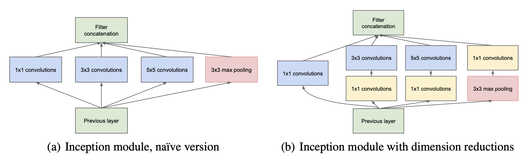
The inception module on the left-hand-side in the picture above has been the original (or naive) version. The problem with this version is that particularly in the case of filters of larger size (\(5 \times 5\)) and a high-dimensional input[1], the number of required learnable parameters and thus the memory- and computation-complexity is high. E.g. for a single filter of size (\(5 \times 5\)), which operates on a 128-dimensional input has \(5 \cdot 5 \cdot 128 = 3200\) parameters (coefficients). Therefore, the inception-module on the right-hand-side of the picture above has been developed. It contains \(1 \times 1\)-convolution for dimensionality reduction.
The configuration of the GoogLeNet, as introduced in [SLJ+14] is given in the table below:
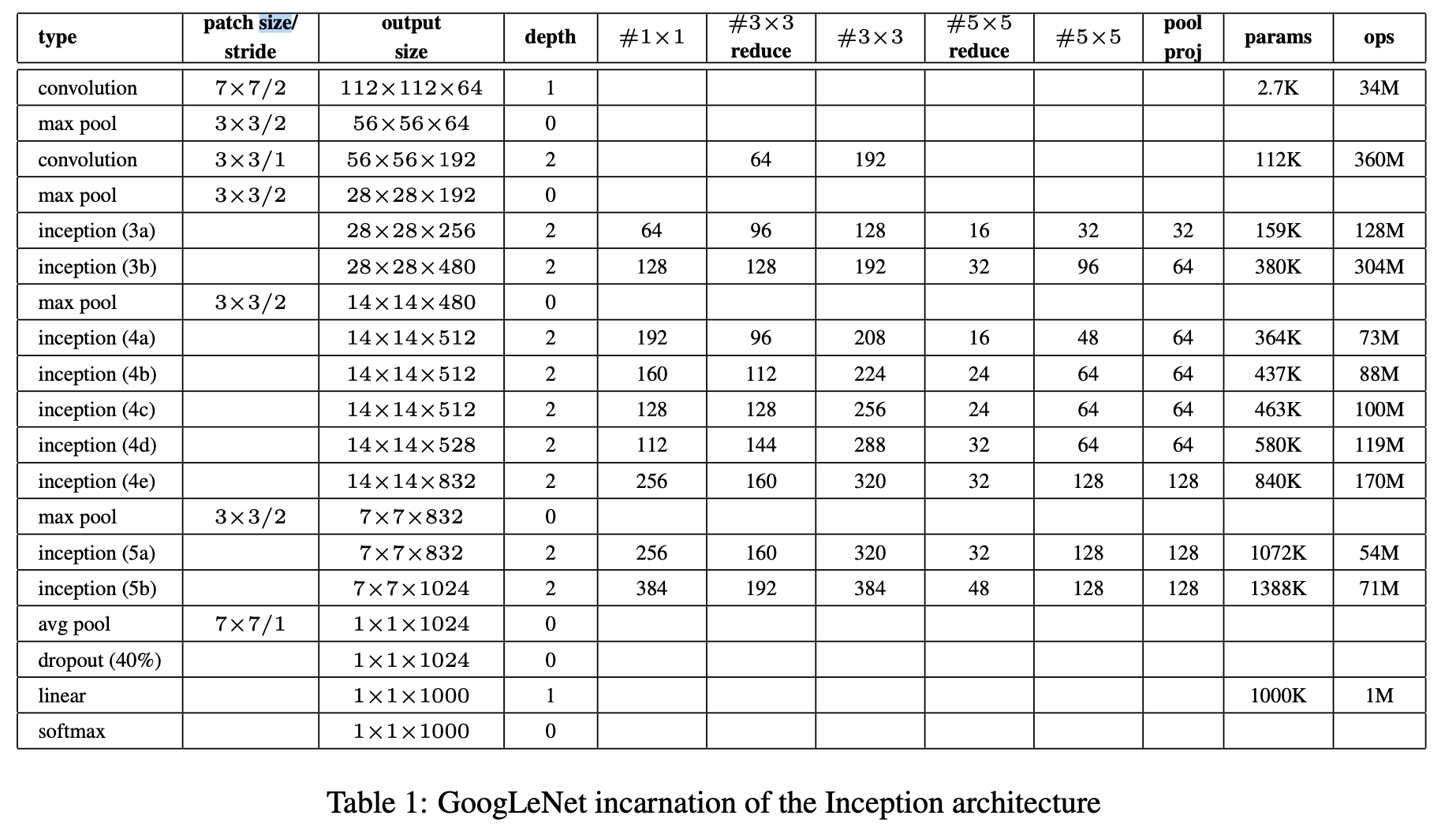
The approach, which won the ILSVRC image classification contest was actually an ensemble of 7 networks - 6 of the type as depicted in the table above + one even wider network. These models were trained with the same data and learning parameters but different sampling policies (cropping from training data and different order in batches).
Moreover, from each test-image 144 different crops have been obtained. The softmax-probabilities of the different crops have been averaged to obtain the final prediction.

ResNet
ResNet has been introduced 2015 in [HZRS16]. The research question underlying this work is
Is learning better networks as easy as stacking more layers?
Recent work has shown that deeper networks perform better, e.g. VGG ([KS14]). But is this true even for very deep networks?
The researchers found the following answer:
Stacking more and more layers together yields degrading performance if conventional approach is applied. However, with the new concept of residual nets, performance increases with increasing depth
They applied their new concept in a very deep neural network, the ResNet with 152 layers. ResNet won ILSVRC 2015 classification task with \(3.57\%\) top-5 error rate. The fact that ResNet also won several other competitions on other dataset proves the generic applicability of the concept.
At the beginning of their research, the authors analysed the performance of CNNs in dependance of an increasing depth. The result is depicted in the plots below. As can be seen the 56-layer network performs worse than the 20-layer network. And this performance decrease is not due to overfitting, because the deeper network is not only worse on test- but also on training-data. Moreover, their networks already integrated Batch Normalization ([IS15]), i.e. the vanishing gradient problem should not be the reason for the bad performance of the deep network.

This result is surprising, because the functions, which can be learned by a shallower network, shall constitute a subspace of the space, which contains all functions that can be learned from a deeper network. For example consider the following construction of a deeper network from a shallower one:
Copy the weights from the shallower network,
learning the identity in the remaining layers
A network, which is constructed in this way should not perform worse than the shallow network.

However, experiments proved that deeper network constructed in this way actually perform worse. Thus one can hypothesize, that
it is not that easy to learn the identity mapping with several layers, or more general: Some function-types are easier to learn than others.
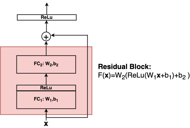
The authors wondered whether it might be easier to learn the target mapping \(H(\mathbf{x})\) or the residual mapping \(F(\mathbf{x})=H(\mathbf{x})-\mathbf{x}\)? For this they introduced the residual block as shown in the image below:

Residual blocks contain short-cut connections and learn \(F(\mathbf{x})\) instead of \(H(\mathbf{x})\). Shortcut-connections do not contain learnable parameters. Stochastic Gradient Descent (SGD) and backpropagation can be applied for residual blocks in the same way as for conventional nets.
A Residual block can consist of an arbitrary number of layers (2 or 3 layers are convenient) of arbitrary type (FC,Conv) and arbitrary activation functions:
In general a single building block in a residual net calculates \(\mathbf{y}\) from it’s input \(\mathbf{x}\) by:
where \(W_i\) and \(b_i\) are the weights-matrix and the bias-vector in the i.th layer of this block. In this case the dimensions of the output \(\mathbf{y}\) and the input \(\mathbf{x}\) must be the same. If the output and input shall have different dimensions, the input can be transformed by \(W_s\):
For the design of \(W_s\) the following options exist:
Option A: Use zero-padding shortcuts for increasing dimensions
Option B: Projection shortcuts are used for increasing dimensions and identity for the others
Option C: All shortcuts are projections
In the ResNet architecture-figure below, such dimension-modifying shortcuts are represented by dotted lines.


Comparison of ResNet and conventional CNN:

Comparison of different dimension-increasing options:

Ensemble: Combination of 6 models of different depth (only 2 of them of depth 152)::

Comparison on ILSVRC
