Similarity Measures¶

Author: Johannes Maucher
Last update: 15th February 2021

In many computer vision tasks it is necessary to compare the similarity between images and image-regions. In the introduction of image features global-, subwindow- and local- image descriptors have been distinguished. Independent of this descriptor type, each descriptor is a numeric vector. Hence, in order to compare image(-regions) we need methods to calculate the similarity of numeric vectors. Actually there exists a bunch of different similarity-measures. The most important of them are defined in this section.

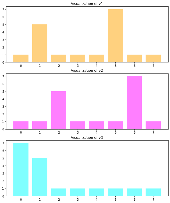
Motivation: Given the following 3 vectors v1, v2 and v3, the question is:

Is v1 or v3 more similar to v2?

import numpy as np
np.set_printoptions(precision=3)
v1=np.array([1,5,1,1,1,7,1,1])
print("v1 = ",v1)
v2=np.array([1,1,5,1,1,1,7,1])
print("v2 = ",v2)
v3=np.array([7,5,1,1,1,1,1,1])
print("v3 = ",v3)

v1 =  [1 5 1 1 1 7 1 1]
v2 =  [1 1 5 1 1 1 7 1]
v3 =  [7 5 1 1 1 1 1 1]

The 3 vectors are visualized below:

from matplotlib import pyplot as plt
plt.figure(figsize=(10,12))
plt.subplot(3,1,1)
plt.bar(np.arange(0,8),v1,color="orange",alpha=0.5)
plt.title("Visualization of v1")
plt.subplot(3,1,2)
plt.bar(np.arange(0,8),v2,color="magenta",alpha=0.5)
plt.title("Visualization of v2")
plt.subplot(3,1,3)
plt.bar(np.arange(0,8),v3,color="cyan",alpha=0.5)
plt.title("Visualization of v3")
plt.show()

Similarity and Distance¶

The similarity between a pair of vectors \(\mathbf{u}=(u_0,u_1,\ldots,u_{N-1})\) and \(\mathbf{v}=(v_0,v_1,\ldots,v_{N-1})\), each of length \(N\), is denoted by

\[ s(\mathbf{u},\mathbf{v}). \]

The distance between the same pair of vectors is denoted by

\[ d(\mathbf{u},\mathbf{v}). \]

Distance and similarity are inverse to each other, i.e. the higher the distance the lower the similarity between anc vice versa. Below the most important distance- and similarity-measures are described. Some of them are primarily defined as distance-metric (e.g. euclidean distance) and a transformation-function can be applied to compute the associated similarity. Others are primarily defined as similarity-metric (e.g. cosine similarity) and a transformation function can be applied to compute the associated distance.

In the context of this section vectors represent Histograms. However, the distance metrics described below can be applied for arbitrary numeric vectors.

We denote by

\[ H_q = \left(H_q(0),H_q(1),H_q(2),\ldots,H_q(N) \right) \]

the N-bin histogram of an image(-region) \(q\). The value \(H_q(i)\) is the frequency of the values in \(q\), which fall into the \(i.th\) bin.

Normalized Histogram:

A normalized representation \(H^n_q\) of histogram \(H_q\) can be obtained as follows:

(2)¶\[ H^n_q := \frac{1}{m_q} \left(H_q(0),H_q(1),H_q(2),\ldots,H_q(Z) \right), \]

where

\[ m_q=\sum\limits_{i=1}^Z H_q(i) \]

Common Distance- and Similarity Metrics¶

Euclidean Distance¶

The Euclidean distance between two histograms \(H_q\) and \(H_p\) is

\[ d_E(H_q,H_p)=\sqrt{\sum_i (H_q(i)-H_p(i))^2} \]

The corresponding similarity measure is

\[ s_E(H_q,H_p)=\frac{1}{d_E(H_q,H_p)+\epsilon}, \]

where \(\epsilon\) is a small value \(>0\), used to avoid zero-division.

Characteristics of the Euclidean distance \(d_E(H_q,H_p)\) are:

Value range: In general \([0,\infty[\).
All bins are weighted equally
Strong impact of outliers
Bin-by-Bin comparison. Drawback: If two images are identical up to a small brightness change, then the histograms look similar up to a small shift along the x-axis (see \(v1\) and \(v2\) in the example above). However, such a type of similarity can not be measured by a Bin-by-Bin metric.

Cosine Similarity¶

The Cosine similarity between two histograms \(H_q\) and \(H_p\) is

\[ s_C(H_q,H_p)= \frac{\sum_i H_q(i)\cdot H_p(i)}{\sqrt{\sum_i H_q(i)^2 \cdot \sum_i H_p(i)^2}}, \]

The corresponding distance measure is

\[ d_C(H_q,H_p)=1-s_C(H_q,H_p) \]

Characteristics of the Cosine similarity \(s_C(H_q,H_p)\):

Value range: \([-1,1]\)
Bin-by-bin comparison
Regards the angle between vectors. Two vectors are maximal similar, if they point to the same direction (the angle between them is 0°).

Pearson Correlation¶

The Pearson correlation (similarity measure) between two histograms \(H_q\) and \(H_p\) is

\[ s_P(H_q,H_p)= \frac{\sum_i (H_q(i)-\mu_q)\cdot (H_p(i)-\mu_p)}{\sqrt{\sum_i (H_q(i)-\mu_q)^2 \cdot \sum_i (H_p(i)-\mu_p)^2}}, \]

where

\[ \mu_q = \frac{1}{N} \sum\limits_{i=1}^N H_q(i) \]

is the mean value over all bins in \(H_q\).

The corresponding distance measure is

\[ d_P(H_q,H_p)=1-s_P(H_q,H_p) \]

Characteristics of the Pearson correlation \(s_P(H_q,H_p)\):

Value range: \([-1,1]\)
Bin-by-bin comparison
Ignores different offsets and is an measure for linearity

Bray-Curtis Distance¶

The Bray-Curtis distance between two histograms \(H_q\) and \(H_p\) is

\[ d_{BC}(H_q,H_p)=\frac{\sum_i |H_q(i)-H_p(i)|}{\sum_i|H_q(i)+H_p(i)|} \]

The corresponding similarity measure is

\[ s_{BC}(H_q,H_p)=1-d_{BC}(H_q,H_p) \]

Characteristics:

Value range: \([0,1]\) for positive signals as in the case of histograms
Bin-by-bin comparison
More robust w.r.t. outliers than euclidean distance
Each bin difference is weighted equally

Canberra Distance¶

The Canberra distance between two histograms \(H_q\) and \(H_p\) is

\[ d_{Ca}(H_q,H_p)=\sum_i\frac{|H_q(i)-H_p(i)|}{|H_q(i)|+|H_p(i)|} \]

The corresponding similarity measure is

\[ s_{Ca}(H_q,H_p)=1-d_{Ca}(H_q,H_p) \]

Characteristics:

Value range: \([0,1]\)
Bin-by-bin comparison
Compared to Bray-Curtis now each bin difference is weighted individually.

Bhattacharyya Distance¶

The Bhattacharyya distance between two normalized histograms \(H^n_q\) and \(H^n_p\) is

\[ d_{Ba}(H^n_q,H^n_p)= \sqrt{1-\sum_i \sqrt{H^n_q(i) \cdot H^n_p(i)}} \]

Characteristics:

Value range: \([0,1]\)
Bin-by-bin comparison
Requires normalized inputs
Statistically motivated for measuring similarity between probability distributions. Here applied for the univariate case, but also applicable for multivariate distributions.

Chi-Square Distance¶

The Chi-Square (\(\chi^2\)) distance between two histograms \(H_q\) and \(H_p\) is

\[ d_{\chi^2}(H_q,H_p)=\sum_i \frac{(H_q(i)-H_p(i))^2}{H_q(i)+H_p(i)} \]

The corresponding similarity measure is

\[ s_{\chi^2}(H_q,H_p)=\frac{1}{d_{\chi^2}(H_q,H_p)+\epsilon}, \]

where \(\epsilon\) is a small value \(>0\), used to avoid zero-division.

Characteristics:

Value range: \([0,\infty]\)
Bin-by-bin comparison
Each bin is weighted individually
Statistically motivated for measuring similarity between probability distributions. Here applied for the univariate case, but also applicable for multivariate distributions.

Intersection Distance¶

The Intersection distance between two histograms \(H_q\) and \(H_p\) is

\[ d_{IS}(H_q,H_p)=\sum_i \min(H_q(i),H_p(i)) \]

The corresponding similarity measure is

\[ s_{IS}(H_q,H_p)=\frac{1}{d_{IS}(H_q,H_p)+\epsilon}, \]

where \(\epsilon\) is a small value \(>0\), used to avoid zero-division.

Characteristics:

Histograms shall be normalized
Value range is \([0,\infty]\)
Bin-by-bin comparison
Measures intersection of both histograms
Introduced in [SB91] for color histogram comparison

Earth Mover Distance (Wasserstein Distance)¶

All of the distance measures introduced so far, ingore shift-similarity. Shift-similar means, that one histogram is the shifted version of the other. This is actually the case for vectors \(v1\) and \(v2\) in the example above. The previously defined distance measure compare bin-by-bin. Therefore, they are not able to detect the shift-similarity.

The Earth Mover Distance (EMD) has been introduced in [RubnerTomasiGuibas98]. It’s not a bin-by-bin similarity measure and it is capable to detect shift-similarity. The drawback of the EMD is that it is quite complex to calculate.

The EMD between two histograms measures the amount of work, which is necessary to transform one histogram to the other, where work is the product of

\[ \mbox{amount of pieces that must be shifted} \cdot \mbox{distance of corresponding shift}. \]

The idea is sketched in the pictures below:

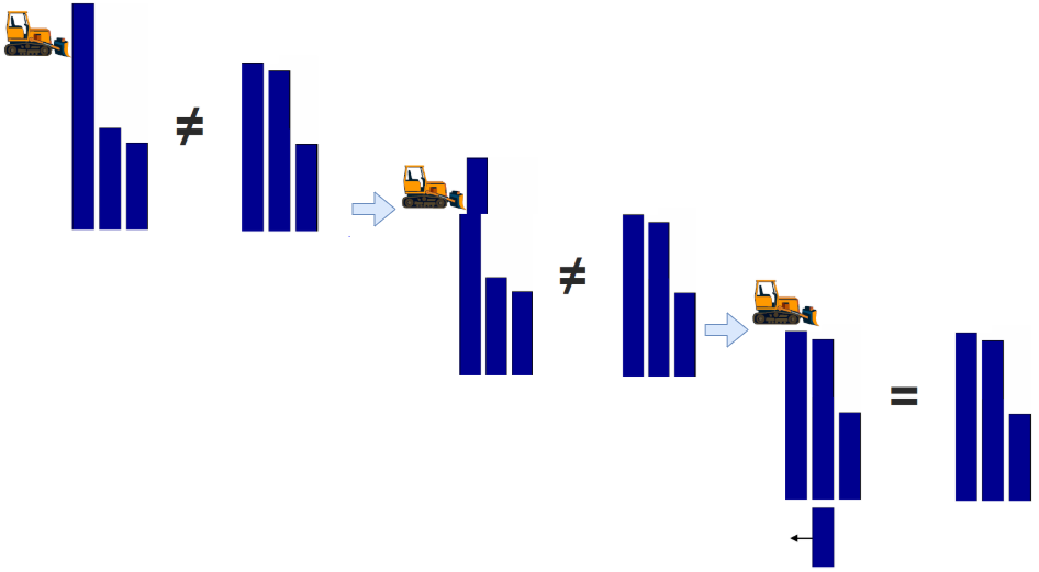
The EMD requires the two histograms to be normalized, i.e. both histograms contain the equal amount of earth.

\[ Work = \sum (\mbox{ distance moved }) \cdot (\mbox{ amount moved }) \]

(3)¶\[ Work = \sum\limits_{a=1}^m \sum\limits_{b=1}^n d_{a,b} \cdot f_{a,b} \]

where \(m\) is the number of bins in histogram \(H_p\) and \(n\) is the number of bins in histogram \(H_q\).

The Earth Mover Distance \(d_{emd}(H_q,H_p)\) between histogram \(H_q\) and histogram \(H_p\) is the minimum possible amount of work, required to convert \(H_p\) into \(H_q\), divided by the sum over all \(f_{a,b}\):

(4)¶\[ Work = \frac{\sum\limits_{a=1}^m \sum\limits_{b=1}^n d_{a,b} \cdot f_{a,b}}{\sum\limits_{a=1}^m \sum\limits_{b=1}^n f_{a,b}} \]

The EMD is also called Wasserstein-Distance (see Wikipedia). A nice example for calculating the EMD between two 2-dimensional distributions can be found here.

Calculation of EMD (Wasserstein-Distance) with scipy¶

In order to calculate the Wasserstein-distance the scipy method wasserstein_distance can be applied. This function calculates a variant of the EMD by:

The histograms are internally normalized, such that in both histograms the sum over all bins is 1 (like in equation (2) ).
Work is calculated as in equation (3), i.e. not normalized like in (4).

Below, we apply this scipy-method to calculate the Wasserstein-distance between \(v1\), \(v2\) and \(v3\):

print("v1 = ",v1)
print("v2 = ",v2)
print("v3 = ",v3)

v1 =  [1 5 1 1 1 7 1 1]
v2 =  [1 1 5 1 1 1 7 1]
v3 =  [7 5 1 1 1 1 1 1]

In order to calculate the EMD, the vectors \(v1\), \(v2\) and \(v3\) are not sufficient, because these vectors contain only frequencies of 8 different values. It is clear that also the values must be defined. Here, we assume that

the first frequency (1 in \(v1\)) is the frequency of the value \(0\) in the first distribution
the second frequency (5 in \(v1\)) is the frequency of the value \(1\) in the first distribution
…
the last frequency (1 in \(v1\)) is the frequency of the value \(7\) in the first distribution

We assume that for all 3 distributions we have the same set of 8 values and define them below:

values=list(range(8))
values

[0, 1, 2, 3, 4, 5, 6, 7]

Then the pairwise Wasserstein-distances between \(v1\), \(v2\) and \(v3\) can be calculated as follows:

from scipy.stats import wasserstein_distance

dw12=wasserstein_distance(values,values,v1,v2)
print("Wasserstein distance between v1 and v2 : %2.3f"%dw12)
dw13=wasserstein_distance(values,values,v1,v3)
print("Wasserstein distance between v1 and v3 : %2.3f"%dw13)
dw23=wasserstein_distance(values,values,v2,v3)
print("Wasserstein distance between v2 and v3 : %2.3f"%dw23)

Wasserstein distance between v1 and v2 : 0.556
Wasserstein distance between v1 and v3 : 1.667
Wasserstein distance between v2 and v3 : 2.222

Let’s check the internal calculation by the example of \(v1\) and \(v2\):

As mentioned above, the scipy-method internally first normalizes the histograms:

v1norm=1/np.sum(v1)*v1
v1norm

array([0.056, 0.278, 0.056, 0.056, 0.056, 0.389, 0.056, 0.056])

v2norm=1/np.sum(v2)*v2
v2norm

array([0.056, 0.056, 0.278, 0.056, 0.056, 0.056, 0.389, 0.056])

Next, in order to transform the normed \(v1\) into the normed \(v2\)
1. an amount of \(4/18\) must be shifted over a distance of \(1\) from bin 1 to bin 2.
2. an amount of \(6/18\) must be shifted over a distance of \(1\) from bin 5 to bin 6.
The calculated Wasserstein distance is then

\[ \frac{4}{18} \cdot 1 + \frac{6}{18} \cdot 1 = \frac{10}{18} = 0.555 \]

Application of different Distance Metrics¶

Below, we will apply all the distance measures introduced above on the pairwise similarity determination between our example-vectors vectors \(v1\), \(v2\) and \(v3\).

The Scipy package spatial.distance contains methods for calculating the euclidean-, Pearson-Correlation-, Canberra- and Bray-Curtis-distance. As already mentioned the EMD distance is implemented as wasserstein_distance() in scipy.stats. The remaining distance measures as well as a corresponding normalization function are defined in this python program.

def normalize(a):
    s=np.sum(a)
    return a/s

def mindist(a,b):
    return 1.0/(1+np.sum(np.minimum(a,b)))

def bhattacharyya(a,b): # this is acutally the Hellinger distance,
                        # which is a modification of Bhattacharyya
                        # Implementation according to http://en.wikipedia.org/wiki/Bhattacharyya_distance
    anorm=normalize(a)
    bnorm=normalize(b)
    BC=np.sum(np.sqrt(anorm*bnorm))
    if BC > 1:
        #print BC
        return 0
    else:
        return np.sqrt(1-BC)

def chi2(a,b):
    idx=np.nonzero(a+b)
    af=a[idx]
    bf=b[idx]
    return np.sum((af-bf)**2/(af+bf))

from scipy.spatial.distance import *
from scipy.stats import wasserstein_distance

methods=[euclidean,correlation,canberra,braycurtis,mindist,bhattacharyya,chi2,wasserstein_distance]
methodName=["euclidean","correlation","canberra","braycurtis","intersection","bhattacharyya","chi2","emd"]

import pandas as pd
distDF=pd.DataFrame(index=methodName,columns=["v1-v2", "v1-v3", "v2-v3"])

values = np.arange(0,len(v1))
for j,m in enumerate(methods):
    if j == len(methods)-1:
       distDF.loc[methodName[j],"v1-v2"]=wasserstein_distance(values,values,v1,v2)
       distDF.loc[methodName[j],"v1-v3"]=wasserstein_distance(values,values,v1,v3)
       distDF.loc[methodName[j],"v2-v3"]=wasserstein_distance(values,values,v2,v3)
    else: 
       distDF.loc[methodName[j],"v1-v2"]=m(v1,v2)
       distDF.loc[methodName[j],"v1-v3"]=m(v1,v3)
       distDF.loc[methodName[j],"v2-v3"]=m(v2,v3)
distDF

	v1-v2	v1-v3	v2-v3
euclidean	10.198039	8.485281	10.198039
correlation	1.316456	0.911392	1.316456
canberra	2.833333	1.500000	2.833333
braycurtis	0.555556	0.333333	0.555556
intersection	0.111111	0.076923	0.111111
bhattacharyya	0.485132	0.387907	0.485132
chi2	14.333333	9.000000	14.333333
emd	0.555556	1.666667	2.222222

The absolute distance values of different distance-measures can not be compared. But we can analyse the for each distance measure the relative distances.

As can be seen all distance measures, except EMD, calculate the same distance between \(v1\) and \(v2\) as between \(v2\) and \(v3\). This is because these distance measures perform a bin-by-bin comparison, and these bin-by-bin comparisons are identical for both vector-pairs. Moreover, all metrics except EMD, find that \(v1\) is closer to \(v3\) than to \(v2\). This contradicts the subjective assessment, because subjectively one would say \(v2\) is closer to \(v1\), because \(v2\) is just a one-step-right-shift of \(v1\).

As will be demonstrated in the next section, the performance of, e.g. a CBIR system, strongly depends on the choice of the distance metric. The question on which metric will perform best in a given task and given data can not be determined in advance, it must be determined empirically.

Global Image Features Histogram-based Image Retrieval

Object Recognition Lecture

Similarity Measures¶

Similarity and Distance¶

Common Distance- and Similarity Metrics¶

Euclidean Distance¶

Cosine Similarity¶

Pearson Correlation¶

Bray-Curtis Distance¶

Canberra Distance¶

Bhattacharyya Distance¶

Chi-Square Distance¶

Intersection Distance¶

Earth Mover Distance (Wasserstein Distance)¶

Calculation of EMD (Wasserstein-Distance) with scipy¶

Application of different Distance Metrics¶