
Histogram-based Image Retrieval
As introduced in Swain, Ballard ([SB91]) 3-dimensional color histograms can be applied for specific object recognition. We consider the image retrieval case, i.e. given a large database of images and a novel query image, the task is to determine the database image which is most similar to the query image. The images in the database as well as the query image are represented by their 3-dimensional color histograms. Hence, the search for the most similar image in the database is equal to find the 3-d color histogram, which matches best to the 3-d color historgram of the query image.
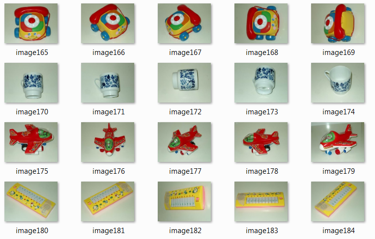
In this demo the Another 53 objects database is applied. The database contains for each of the 53 objects 5 images, which differ in viewpoint, rotation vertical- and horizontal alignment of the object. Actually, the dataset contains one object, for which only one image exists. This image (image215) has been removed for the test below. A sample of the image database is shown in the picture below.
Testprocedure
In order to evaluate the recognition performance of the 3-d color histogram image retrieval system a leave-one-out test procedure is applied. This means that in each of the 265 iterations one image is selected as query image and the remaining 264 images constitute the database. The recognition is considered to be correct, if the best matching image contains the same object as the query image.
Recognition performance depends on the metric used for comparing multidimensional histograms. In this demo the following distance measures are compared:
Euclidean
Pearson Correlation
Canberra
Bray-Curtis
Intersection
Bhattacharyya
Chi-Square
For a formal definition of these metrics see previous section.
Implementation
The following modules are applied:
import os
import numpy as np
from PIL import Image
import cv2
from scipy.spatial.distance import *
from scipy.stats import wasserstein_distance
Distance functions
The Scipy package spatial.distance contains methods for calculating the euclidean-, Pearson-Correlation-, Canberra- and Bray-Curtis-distance. The remaining distance measures as well as a corresponding normalization function are defined in this python program.
def normalize(a):
    s=np.sum(a)
    return a/s

def mindist(a,b):
    return 1.0/(1+np.sum(np.minimum(a,b)))

def bhattacharyya(a,b): # this is acutally the Hellinger distance,
                        # which is a modification of Bhattacharyya
                        # Implementation according to http://en.wikipedia.org/wiki/Bhattacharyya_distance
    anorm=normalize(a)
    bnorm=normalize(b)
    BC=np.sum(np.sqrt(anorm*bnorm))

    if BC > 1:
        #print BC
        return 0
    else:
        return np.sqrt(1-BC)

def chi2(a,b):
    idx=np.nonzero(a+b)
    af=a[idx]
    bf=b[idx]
    return np.sum((af-bf)**2/(af+bf))
The applied metrics are defined as a list of function names and as a list of strings:
methods=[euclidean,correlation,canberra,braycurtis,mindist,bhattacharyya,chi2,wasserstein_distance]
methodName=["euclidean","correlation","canberra","braycurtis","intersection","bhattacharyya","chi2","emd"]
Next, the number of bins per dimension B is defined. The 3-dimensional color histogram then consists of \(B\cdot B\cdot B\) bins. The images are imported from the locally saved image database, which contains the 265 .jpeg images. For calculating the 3-dimensional color histograms of the images the Numpy method histogramdd is applied. The histograms are normalized and flattened (transformed into a 1-dimensional array)
B=5
# create a list of images
path = '../Data/66obj/images'
imlist = [os.path.join(path,f) for f in os.listdir(path) if f.endswith(".JPG")]
imlist.sort()
#print(imlist)
features = np.zeros([len(imlist), B*B*B])
hists=[]
for i,f in enumerate(imlist):
    im = np.array(Image.open(f))
    # multi-dimensional histogram
    h=cv2.calcHist([im],[0,1,2],None,[B,B,B],[0,256,0,256,0,256])
    h=normalize(h) #normalization
    features[i] = h.flatten()
    hists.append(h)
print(features.shape)
N_IM=features.shape[0]
(265, 125)
import pandas as pd
resultDF=pd.DataFrame(index=methodName,columns=["Correct", "Error"])
resultDF
| Correct | Error | |
|---|---|---|
| euclidean | NaN | NaN |
| correlation | NaN | NaN |
| canberra | NaN | NaN |
| braycurtis | NaN | NaN |
| intersection | NaN | NaN |
| bhattacharyya | NaN | NaN |
| chi2 | NaN | NaN |
| emd | NaN | NaN |
The following outer loop iterates over all distance-metrics defined in list methods. For each metric first the distance for all pairs of images is calculated and stored in the 2-dimensional array dist. The entry in row i, column j of this matrix stores the distance between the histograms of the i.th and the j.th image. Applying numpy’s argsort() method on each row of the 2 dimensional array dist another 2-dimensional array s is calculated. The i.th row of this matrix contains the indicees of all images, sorted w.r.t. increasing distance to image i. I.e. in the first column of the i.th row of s is the index i and in the second column is the index of the image, which matches best with image i. In order to determine if the recognition is correct, one must just check if the index in the second column of s belongs to the same object as the index of the corresponding row. This can be done by a simple integer division, since the images are indexed such that indicees 0 to 4 belong to the same object, indicees 5 to 9 belong to the next object, and so on. The results are saved in the pandas dataframe.
values = np.arange(0,features.shape[1])
for j,m in enumerate(methods):
    dist=np.zeros((N_IM,N_IM))
    for h1 in range(N_IM):
        for h2 in range(h1,N_IM):
           if j == len(methods)-1:
            dist[h1,h2]=wasserstein_distance(values,values,features[h1,:],features[h2,:])
           else:
            dist[h1,h2]=m(features[h1,:],features[h2,:])
           dist[h2,h1]=dist[h1,h2]
    s=np.argsort(dist,axis=1)
    correct=0
    error=0
    for i in range(N_IM):
        for a in s[i,1:2]:
            if int(a/5) != int(i/5):
                error+=1
            else:
                correct+=1
    resultDF.loc[methodName[j],"Correct"]=correct
    resultDF.loc[methodName[j],"Error"]=error
resultDF
| Correct | Error | |
|---|---|---|
| euclidean | 181 | 84 |
| correlation | 175 | 90 |
| canberra | 257 | 8 |
| braycurtis | 222 | 43 |
| intersection | 222 | 43 |
| bhattacharyya | 243 | 22 |
| chi2 | 239 | 26 |
| emd | 159 | 106 |
Use pretrained CNNs for Retrieval
Convolutional Neural Networks (CNN) consist of a feature-extractor part and a classifier. The last part of the CNN (blue part in the image below) is the classifier, consisting one or more dense layers. All other layers (orange part in the image below) constitute the feature extractor part, usually realised by convolutional and pooling layers.
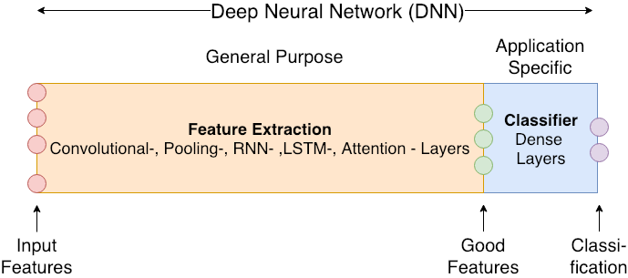 In a well trained CNN, the feature-extractor part provides a good representation of the input image to the classifier.
In the context of image retrieval one can apply the pretrained feature-extractor part to calculate a good representation of all images - hopefully this representation is better than e.g. a global color-histogram. Instead of comparing color histograms of images in order to find the best matching image, one can compare these dnn-generated features for image retrieval.
In the remainder of this notebook we apply different pretrained deep neural networks to calculate good representations. Based on these representations best matching image-pairs are determined in the same way as above. All CNNs have been pretrained on the imagenet-dataset.
from tensorflow.keras.applications import vgg16, inception_v3, resnet50, mobilenet
from tensorflow.keras.preprocessing.image import load_img
from tensorflow.keras.preprocessing.image import img_to_array
#from tensorflow.keras.applications.imagenet_utils import decode_predictions
import matplotlib.pyplot as plt
Load pretrained CNNs without the classifier part, i.e. only the feature-extractor part:
vgg_model = vgg16.VGG16(weights='imagenet',include_top=False)
inception_model = inception_v3.InceptionV3(weights='imagenet',include_top=False)
resnet_model = resnet50.ResNet50(weights='imagenet',include_top=False)
mobilenet_model = mobilenet.MobileNet(weights='imagenet',include_top=False)
WARNING:tensorflow:`input_shape` is undefined or non-square, or `rows` is not in [128, 160, 192, 224]. Weights for input shape (224, 224) will be loaded as the default.
IMGSIZE_X=224
IMGSIZE_Y=224
image_batch=np.zeros((len(imlist),IMGSIZE_X,IMGSIZE_Y,3))
for i,filename in enumerate(imlist):
    #im = np.array(Image.open(f))
    original = load_img(filename, target_size=(IMGSIZE_X,IMGSIZE_Y))
    numpy_image = img_to_array(original)
    image_batch[i,:,:,:] = np.expand_dims(numpy_image, axis=0)
print(image_batch.shape)
(265, 224, 224, 3)
nets=[vgg16, inception_v3, resnet50, mobilenet]
models=[vgg_model, inception_model, resnet_model, mobilenet_model]
modelNames=["vgg","inception","resnet","mobilenet"]
import pandas as pd
resultDF2=pd.DataFrame(index=modelNames,columns=["Correct", "Error"])
resultDF2
| Correct | Error | |
|---|---|---|
| vgg | NaN | NaN |
| inception | NaN | NaN |
| resnet | NaN | NaN |
| mobilenet | NaN | NaN |
metric=correlation #euclidean
for net,model,name in zip(nets,models,modelNames):
    processed_image = net.preprocess_input(image_batch.copy())
    predictions = model.predict(processed_image)
    features=predictions.reshape(265,-1)
    #modelDict[name]["features"]=features

    dist=np.zeros((N_IM,N_IM))
    for h1 in range(N_IM):
        for h2 in range(h1,N_IM):
           dist[h1,h2]=metric(features[h1,:],features[h2,:])
           dist[h2,h1]=dist[h1,h2]
    s=np.argsort(dist,axis=1)
    correct=0
    error=0
    for i in range(N_IM):
        for a in s[i,1:2]:
            if int(a/5) != int(i/5):
                error+=1
            else:
                correct+=1
    resultDF2.loc[name,"Correct"]=correct
    resultDF2.loc[name,"Error"]=error
    #print("Name: %s: \t Correct: %3d \t Error: %3d"%(name,correct,error))
resultDF2
| Correct | Error | |
|---|---|---|
| vgg | 248 | 17 |
| inception | 248 | 17 |
| resnet | 260 | 5 |
| mobilenet | 253 | 12 |