Multi-Person 2D Pose Estimation using Part Affinity Fields¶

Author: Johannes Maucher
Last update: 14.06.2018

Pose Estimation requires to detect, localize and track the major parts/joints of the body, e.g. shoulders, ankle, knee, wrist etc.

References:
- Chao et al; Realtime Multi-Person 2D Pose Estimation using Part Affinty Fields. This paper defines the theory of the approach, implemented in this notebook. All images in this notebook are from this paper.
- Video from the authors
- https://www.learnopencv.com/deep-learning-based-human-pose-estimation-using-opencv-cpp-python/
Datasets:
Pretrained Caffe models:
- Pretrained Caffe model for MPII
- Pretrained Caffe model for COCO

#!pip install opencv-python==3.4.13.47

import cv2
import time
import numpy as np
import matplotlib.pyplot as plt
%matplotlib inline

print(cv2.__version__)

3.4.13

Multiperson Pose Estimation¶

Approaches for Multi-Person Pose Estimation¶

Top-Down¶

Person Detection
Single Person Pose Estimation

Bottom-Up¶

Detect keypoints (joints) in the image
Connect joints to single person pose-models

Theory¶

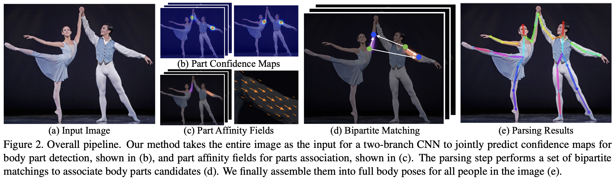
In this notebook a bottom-up approach, which applies deep neural netorks is implemented. The approach has been developed in Chao et al; Realtime Multi-Person 2D Pose Estimation using Part Affinty Fields. All images in this notebook are from this paper.

Overall Pipeline¶

Pass entire image to CNN
CNN predicts in multiple stages increasingly accurate
- confidence maps for body part candidates
- part affinity fields for parts-associations
Perform bipartite matching to find candidates of body-part associations
Assemble parts and associations to full body poses

Confidence Maps and Part Affinitiy Fields¶

Set of $J$ Confidence Maps:

\[ S=\lbrace S_1,S_2,\ldots,S_J \rbrace,$$ one for each body-part. * Set of $C$ Part Affinity Fields: \]

L=\lbrace L_1,L_2,\ldots,L_C \rbrace, $$

one per limb.

Both have the same size $w \times h$ as the image at the input

CNN Architecture¶

Stage 0: First 10 layers of VGG16, pretrained and fine tuned $\Rightarrow$ Feature Extraction
Stage 1:
Stage t ($t\geq2$):

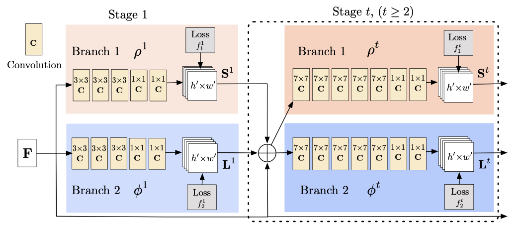
In each stage the simultaneous prediction of Confidence Maps and Part Affinity Fields is refined.
The multi-stage approach mitigates the vanishing gradient problem
Input to the first branch are the features F, extracted from the first 10 layers of VGG16
In each subsequent stage, the predictions from both branches in the previous stage, along with the original image features F, are concatenated and used to produce refined predictions
An L2 loss between the estimated predictions and the groundtruth maps and fields is applied in each stage.

Loss at each stage¶

Loss function for Confidence Map at stage t

\[ f_S^t= \sum\limits_{j=1}^J \sum_{\mathbf{b}} W(\mathbf{p}) \cdot \mid \mid S_j^t(\mathbf{p})-S_j^*(\mathbf{p})\mid\mid ^2) \]

Loss function for Part Affinity Field at stage t

\[ f_L^t= \sum\limits_{c=1}^C \sum_{\mathbf{b}} W(\mathbf{p}) \cdot \mid \mid L_c^t(\mathbf{p})-L_c^*(\mathbf{p})\mid\mid ^2) \]

$S_j^*$ and $L_c^*$ are the groundtruths. $W$ is a binary mask with $W(\mathbf{p})=0$ if annotation is missing at an image location $\mathbf{p}$.

Overall Loss¶

The overall loss function is

\[ f=\sum\limits_{t=1}^T (f_S^t+f_L^t) \]

Stochastic Gradient Descent is applied to minimize the overall loss during training

Groundtrouth for Confidence Maps¶

Put Gaussian peaks over ground truth locations $\mathbf{x_{j,k}}$ of each body part $j$. Value at location $\mathbf{p}$ for the $k.th$ person in $S_{j,k}^*$:

\[ S_{j,k}^*(\mathbf{p}) = \exp \left( - \frac{\mid \mid \mathbf{p} - \mathbf{x_{j,k}} \mid \mid ^2}{\sigma^2} \right). \]

Gaussian peaks of multiple persons in one map may overlap at location $\mathbf{p}$
They are combined by

\[ S_j^*(\mathbf{p}) = \max_k S_{j,k}^*(\mathbf{p}) \]

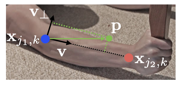
Groundtruth for Part Affinity Fields¶

$\mathbf{x_{j_1,k}}$ and $\mathbf{x_{j_2,k}}$ are the groundtruth-positions of bodyparts $j_1$ and $j_2$ from limb $c$ of person $k$.
$L_{c,k}^*(\mathbf{p})$ is a unit vector

\[ \mathbf{v}=\frac{(\mathbf{x_{j_2,k}}-\mathbf{x_{j_1,k}})}{\mid \mid \mathbf{x_{j_2,k}}-\mathbf{x_{j_1,k}}\mid \mid}, \]

that points from one bodypart to the other, if $\mathbf{p}$ lies on the limb, otherwise it is 0.

$\mathbf{p}$ is said to lie on the limb if

\[ 0 \leq (\mathbf{p}-\mathbf{x_{j_1,k}}) \cdot \mathbf{v}\leq l_{c,k} \]

and

\[ 0 \leq (\mathbf{p}-\mathbf{x_{j_1,k}}) \cdot \mathbf{v_{\perp}}\leq \sigma_l , \]

where $\sigma_l$ is the limb width and $l_{c,k}=\mid \mid \mathbf{x_{j_1,k}}-\mathbf{x_{j_2,k}}\mid \mid$.

Groundtruth for Part Affinity Fields¶

Since the PAFs of multiple persons may overlap, they are combined by

\[ L_c^*(\mathbf{p}) = \frac{1}{n_c(\mathbf{p})} \sum \limits_k L_{c,k}^*(\mathbf{p}) \]

Infer limbs from part candidates¶

Non-maximum suppression is applied on the detected confidence maps to obtain a set of discrete part candidate locations
For each part there may be several candidates, due to
- false positive detections
- multiple persons in the image
Set of part candidate locations defines a large set of possible limbs, among which the true limbs must be detected.
For this the association between part candidates is measured as described in the following slide.

Measure Association between candidate part detections¶

During testing association between candidate part detections is measured

\[ E=\int_{u=0}^{u=1} L_c(\mathbf{p}(u)) \cdot \frac{(\mathbf{d_{j_2,k}}-\mathbf{d_{j_1,k}})}{\mid \mid \mathbf{d_{j_2,k}}-\mathbf{d_{j_1,k}}\mid \mid} du , \]

where $\mathbf{p}(u)$ interpolates the position between the two bodypart-locations $\mathbf{d_{j_1,k}}$ and $\mathbf{d_{j_2,k}}$:

\[ \mathbf{p}(u)=(1-u)\mathbf{d_{j_1,k}} + u \mathbf{d_{j_2,k}} \]

$L_c$ is the predicted PAF for limb $c$ and $\mathbf{d_{j_1,k}}$ and $\mathbf{d_{j_2,k}}$ are predicted part posistions (candidates for being part of limb $c$).

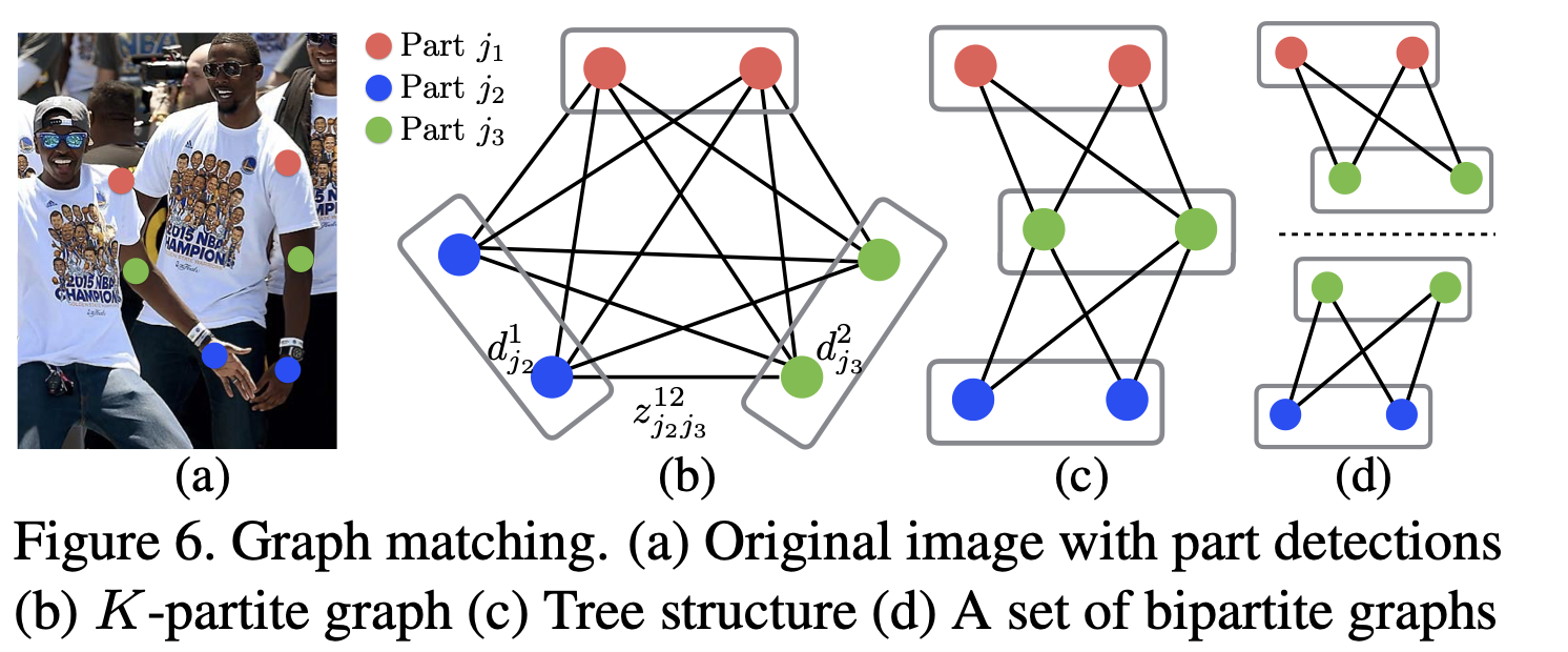
Optimisation problem¶

Set of body-part detection candidates:

\[ D_J = \lbrace \mathbf{d}_j^m : \mbox{ for } j \in \lbrace 1 \ldots J \rbrace, m \in \lbrace 1 \ldots N_j \rbrace \rbrace, \]

where * $N_j$: number of candidates of part $j$ * $\mathbf{d}_j^m$: location of $m.th$ detection candidate for part $j$

Connection indicator

\[ z_{j_1j_2}^{mn} \in \lbrace 0,1 \rbrace, \]

with $z_{j_1j_2}^{mn}=1$, if detection candidates $\mathbf{d}_{j_1}^m$ and $\mathbf{d}_{j_2}^n$ are connected.

Goal ist to find the optimal assignment for the set of all possible connections

\[ Z=\lbrace z_{j_1j_2}^{mn} : \mbox{ for } j_1,j_2 \in \lbrace 1 \ldots J \rbrace, m \in \lbrace 1 \ldots N_{j_1} \rbrace, n \in \lbrace 1 \ldots N_{j_2} \rbrace \rbrace, \]

For a pair of parts $j_1$ and $j_2$ the optimsation problem can be considered as an maximum weight matching problem in a bipartite Graph
A matching in a bipartite graph is a subset of the edges chosen in such a way that no two edges share a node. Our goal is to find a matching with maximum weight for the chosen edges

\[ \max_{Z_c} E_c = \max_{Z_c} \sum\limits_{m \in D_{j_1}} \sum\limits_{n \in D_{j_2}} E_{mn} \cdot z_{j_1j_2}^{mn}, \]

such that

$\forall m \in D_{j_1}: \sum\limits_{n \in D_{j_2}} z_{j_1j_2}^{mn} \leq 1$ and
$\forall n \in D_{j_2}: \sum\limits_{m \in D_{j_1}} z_{j_1j_2}^{mn} \leq 1$

Maximum Weight Matching in Bipartite-Graph¶

Implementation¶

The authors of Chao et al; Realtime Multi-Person 2D Pose Estimation using Part Affinty Fields provide a pretrained model for the pose-estimation approach, which has been descriped in the Theory part of this notebook. This pretrained model will be applied in the following code-cells.

Specify the model to be used¶

COCO and MPI are body pose estimation models. COCO has 18 points and MPI has 15 points as output.
HAND is hand keypoints estimation model. It has 22 points as output.

The provided models have been trained with the Caffe Deep Learning Framework. Caffe models are specified by 2 files:

the .prototxt file specifies the architecture of the neural network
the .caffemodel file stores the weights of the trained model

The .prototxt-files can be downloaded from:

https://github.com/CMU-Perceptual-Computing-Lab/openpose/blob/master/models

The .caffemodel files can be downloaded from:

MODE = "MPI"

if MODE is "COCO":
    protoFile = "./pose/coco/pose_deploy_linevec.prototxt"
    weightsFile = "./pose/coco/pose_iter_440000.caffemodel"
    nPoints = 18
    POSE_PAIRS = [ [1,0],[1,2],[1,5],[2,3],[3,4],[5,6],[6,7],[1,8],[8,9],[9,10],[1,11],[11,12],[12,13],[0,14],[0,15],[14,16],[15,17]]

elif MODE is "MPI" :
    protoFile = "/Users/johannes/DataSets/pose/pose_deploy_linevec_faster_4_stages.prototxt"
    weightsFile = "/Users/johannes/DataSets/pose/pose_iter_160000.caffemodel"
    nPoints = 15
    POSE_PAIRS = [[0,1], [1,2], [2,3], [3,4], [1,5], [5,6], [6,7], [1,14], [14,8], [8,9], [9,10], [14,11], [11,12], [12,13] ]
    

<>:3: SyntaxWarning: "is" with a literal. Did you mean "=="?
<>:9: SyntaxWarning: "is" with a literal. Did you mean "=="?
<>:3: SyntaxWarning: "is" with a literal. Did you mean "=="?
<>:9: SyntaxWarning: "is" with a literal. Did you mean "=="?
<ipython-input-5-a10dad32cb4c>:3: SyntaxWarning: "is" with a literal. Did you mean "=="?
  if MODE is "COCO":
<ipython-input-5-a10dad32cb4c>:9: SyntaxWarning: "is" with a literal. Did you mean "=="?
  elif MODE is "MPI" :

COCO Output Format:

Nose – 0, Neck – 1, Right Shoulder – 2, Right Elbow – 3, Right Wrist – 4, Left Shoulder – 5, Left Elbow – 6, Left Wrist – 7, Right Hip – 8, Right Knee – 9, Right Ankle – 10, Left Hip – 11, Left Knee – 12, LAnkle – 13, Right Eye – 14, Left Eye – 15, Right Ear – 16, Left Ear – 17, Background – 18

MPII Output Format:

Head – 0, Neck – 1, Right Shoulder – 2, Right Elbow – 3, Right Wrist – 4, Left Shoulder – 5, Left Elbow – 6, Left Wrist – 7, Right Hip – 8, Right Knee – 9, Right Ankle – 10, Left Hip – 11, Left Knee – 12, Left Ankle – 13, Chest – 14, Background – 15

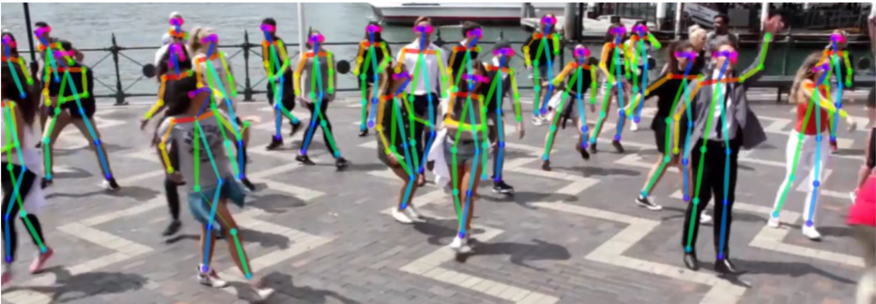
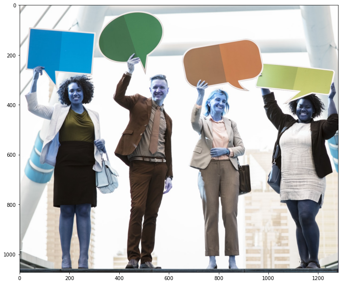
Load image¶

image1 = cv2.imread("multiple.jpeg")
frameWidth = image1.shape[1]
frameHeight = image1.shape[0]
threshold = 0.1

plt.figure(figsize=(12,10))
plt.imshow(image1)
plt.show()

Load pretrained network¶

print(protoFile)
print(weightsFile)

/Users/johannes/DataSets/pose/pose_deploy_linevec_faster_4_stages.prototxt
/Users/johannes/DataSets/pose/pose_iter_160000.caffemodel

net = cv2.dnn.readNetFromCaffe(protoFile, weightsFile)

inWidth = 368
inHeight = 368

Transform image to Caffe blob¶

The image must be converted into a Caffe blob format. This is done using the blobFromImage()-function. The parameters are

the image that shall be converted
The operation to transform each pixel into a float between 0 and 1.
the dimensions of the image
the Mean value to be subtracted (here: (0,0,0)).
a boolean which defines whether R and B channels shall be swapped. Here, there is no need to swapping, because both OpenCV and Caffe use BGR format.

inpBlob = cv2.dnn.blobFromImage(image1, 1.0 / 255, (inWidth, inHeight),
                          (0, 0, 0), swapRB=False, crop=False)

Pass input blob through the network¶

net.setInput(inpBlob)
output = net.forward()

The network’s output contains the following elements:

first dimension: image ID - this is relevant in the case that multiple images are passed to the network.
second dimension: index of a keypoint. The model produces Confidence Maps and Part Affinity maps which are all concatenated. For COCO model it consists of 57 elements – 18 keypoint confidence Maps + 1 background + 19*2 Part Affinity Maps. Similarly, for MPI, it produces 44 points.
third dimension: height of the output map.
fourth dimension: width of the output map.

print(output.shape)
np.set_printoptions(precision=4)
kp=5
print("Confidence map for keypoint {0:d}:".format(kp))
print(output[0, kp, :, :])
print("Maximum in confidence map: {0:1.3f}".
      format(np.max(output[0, kp, :, :])))

(1, 44, 46, 46)
Confidence map for keypoint 5:
[[0.0013 0.0013 0.0011 ... 0.0014 0.0014 0.0015]
 [0.0017 0.0014 0.0011 ... 0.0013 0.0013 0.0014]
 [0.0043 0.0024 0.0011 ... 0.0013 0.0013 0.0013]
 ...
 [0.0015 0.0014 0.0012 ... 0.0011 0.0023 0.0016]
 [0.0015 0.0014 0.0012 ... 0.0011 0.0021 0.0021]
 [0.0034 0.0013 0.0012 ... 0.0018 0.0023 0.0026]]
Maximum in confidence map: 0.833

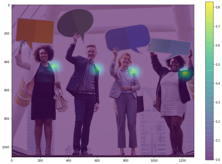
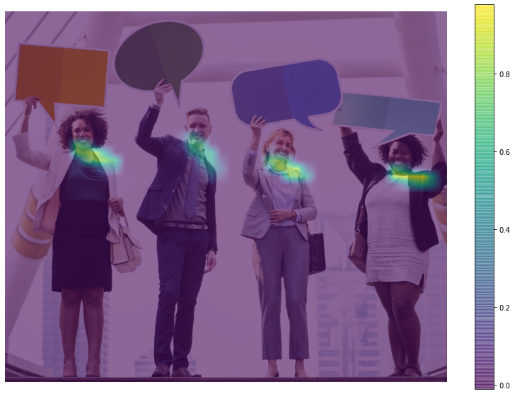
Plot confidence map of selected keypoint¶

kp = 5
probMap = output[0, kp, :, :]
probMap = cv2.resize(probMap, (image1.shape[1], image1.shape[0]))
plt.figure(figsize=[14,10])
plt.imshow(cv2.cvtColor(image1, cv2.COLOR_BGR2RGB))
plt.imshow(probMap, alpha=0.6)
plt.colorbar()
#plt.axis("off")

<matplotlib.colorbar.Colorbar at 0x7fe63d7369a0>

Plot affinity map on the image¶

i = 24
probMap = output[0, i, :, :]
probMap = cv2.resize(probMap, (image1.shape[1], image1.shape[0]))
plt.figure(figsize=[14,10])
plt.imshow(cv2.cvtColor(image1, cv2.COLOR_BGR2RGB))
plt.imshow(probMap, alpha=0.6)
plt.colorbar()
plt.axis("off")

(-0.5, 1279.5, 1071.5, -0.5)

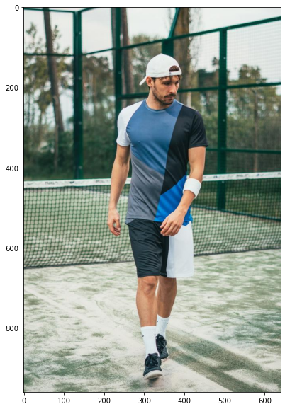
Keypoints of image with only single person¶

frame = cv2.imread("single.jpeg")
frameCopy = np.copy(frame)
frameWidth = frame.shape[1]
frameHeight = frame.shape[0]
threshold = 0.1

plt.figure(figsize=(12,10))
plt.imshow(cv2.cvtColor(frame, cv2.COLOR_BGR2RGB))
plt.show()

Pass image-blob to network¶

inpBlob = cv2.dnn.blobFromImage(frame, 1.0 / 255, (inWidth, inHeight),
                          (0, 0, 0), swapRB=False, crop=False)

net.setInput(inpBlob)

output = net.forward()
H = output.shape[2]
W = output.shape[3]

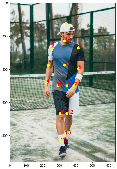
Determine detected part locations¶

The location of each detected keypoint can be obtained by determining the maxima of the keypoint’s confidence map. A threshold is applied to reduce false positive detections. In order to plot the keypoint in the image, it’s location in the output-map must be transformed to the corresponding image location.

# Empty list to store the detected keypoints
points = []

for i in range(nPoints):
    # confidence map of corresponding body's part.
    probMap = output[0, i, :, :]

    # Find global maxima of the probMap.
    minVal, maxVal, minLoc, maxLoc = cv2.minMaxLoc(probMap)
    
    prob=maxVal
    point=maxLoc
    
    # Scale the point to fit on the original image
    x = (frameWidth * point[0]) / W
    y = (frameHeight * point[1]) / H

    if prob > threshold : 
        cv2.circle(frameCopy, (int(x), int(y)), 8, (0, 255, 255), thickness=-1, lineType=cv2.FILLED)
        cv2.putText(frameCopy, "{}".format(i), (int(x), int(y)), cv2.FONT_HERSHEY_SIMPLEX, 1, (0, 0, 255), 2, lineType=cv2.LINE_AA)
        cv2.circle(frame, (int(x), int(y)), 8, (0, 0, 255), thickness=-1, lineType=cv2.FILLED)

        # Add the point to the list if the probability is greater than the threshold
        points.append((int(x), int(y)))
    else :
        points.append(None)

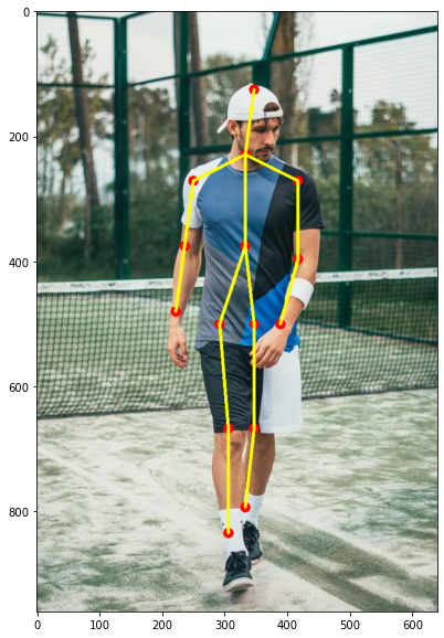
From the detected keypoints and the knowledge of which keypoint maps to which bodypart the skeleton can be drawn. For this the elements of the variable pairs are applied. These elements define which keypoint-pairs define a limb.

plt.figure(figsize=[10,10])
plt.imshow(cv2.cvtColor(frameCopy, cv2.COLOR_BGR2RGB))
plt.show()

for pair in POSE_PAIRS:
    partA = pair[0]
    partB = pair[1]

    if points[partA] and points[partB]:
        cv2.line(frame, points[partA], points[partB], (0, 255, 255), 3)


plt.figure(figsize=[10,10])
plt.imshow(cv2.cvtColor(frame, cv2.COLOR_BGR2RGB))
plt.show()

Face Recognition using FaceNet References

Object Recognition Lecture

Multi-Person 2D Pose Estimation using Part Affinity Fields¶

Multiperson Pose Estimation¶

Approaches for Multi-Person Pose Estimation¶

Top-Down¶

Bottom-Up¶

Theory¶

Overall Pipeline¶

Confidence Maps and Part Affinitiy Fields¶

CNN Architecture¶

Loss at each stage¶

Overall Loss¶

Groundtrouth for Confidence Maps¶

Groundtruth for Part Affinity Fields¶

Groundtruth for Part Affinity Fields¶

Infer limbs from part candidates¶

Measure Association between candidate part detections¶

Optimisation problem¶

Maximum Weight Matching in Bipartite-Graph¶

Implementation¶

Specify the model to be used¶

Load image¶

Load pretrained network¶

Transform image to Caffe blob¶

Pass input blob through the network¶

Plot confidence map of selected keypoint¶

Plot affinity map on the image¶

Keypoints of image with only single person¶

Pass image-blob to network¶

Determine detected part locations¶