
8.4. CNN, LSTM and Attention for IMDB Movie Review classification
Author: Johannes Maucher
Last Update: 23.11.2020
The IMDB Movie Review corpus is a standard dataset for the evaluation of text-classifiers. It consists of 25000 movies reviews from IMDB, labeled by sentiment (positive/negative). In this notebook a Convolutional Neural Network (CNN) is implemented for sentiment classification of IMDB reviews.
import numpy as np
import pandas as pd
from tensorflow.keras.preprocessing.text import Tokenizer
from tensorflow.keras.preprocessing.sequence import pad_sequences
from tensorflow.keras.utils import to_categorical
from tensorflow.keras.layers import Embedding, Dense, Input, Flatten, Conv1D, MaxPooling1D, Dropout, Concatenate, GlobalMaxPool1D
from tensorflow.keras.models import Model
from tensorflow.keras.datasets import imdb
MAX_SEQUENCE_LENGTH = 500  # all text-sequences are padded to this length
MAX_NB_WORDS = 10000        # number of most-frequent words that are regarded, all others are ignored
EMBEDDING_DIM = 100         # dimension of word-embedding
INDEX_FROM=3
8.4.1. Access IMDB dataset
The IMDB dataset is already available in Keras and can easily be accessed by
imdb.load_data().
The returned dataset contains the sequence of word indices for each review.
(X_train, y_train), (X_test, y_test) = imdb.load_data(num_words=MAX_NB_WORDS,index_from=INDEX_FROM)
print(X_train.shape)
print(X_test.shape)
print(y_train.shape)
print(y_test.shape)
(25000,)
(25000,)
(25000,)
(25000,)
X_train[0][:10] #plot first 10 elements of the sequence
[1, 14, 22, 16, 43, 530, 973, 1622, 1385, 65]
The representation of text as sequence of integers is good for Machine Learning algorithms, but useless for human text understanding. Therefore, we also access the word-index from Keras IMDB dataset, which maps words to the associated integer-IDs. Since we like to map integer-IDs to words we calculate the inverse wordindex inv_wordindex:
wordindex=imdb.get_word_index(path="imdb_word_index.json")
wordindex = {k:(v+INDEX_FROM) for k,v in wordindex.items()}
wordindex["<PAD>"] = 0
wordindex["<START>"] = 1
wordindex["<UNK>"] = 2
wordindex["<UNUSED>"] = 3

inv_wordindex = {value:key for key,value in wordindex.items()}
The first film-review of the training-partition then reads as follows:
print(' '.join(inv_wordindex[id] for id in X_train[0] ))
<START> this film was just brilliant casting location scenery story direction everyone's really suited the part they played and you could just imagine being there robert <UNK> is an amazing actor and now the same being director <UNK> father came from the same scottish island as myself so i loved the fact there was a real connection with this film the witty remarks throughout the film were great it was just brilliant so much that i bought the film as soon as it was released for <UNK> and would recommend it to everyone to watch and the fly fishing was amazing really cried at the end it was so sad and you know what they say if you cry at a film it must have been good and this definitely was also <UNK> to the two little boy's that played the <UNK> of norman and paul they were just brilliant children are often left out of the <UNK> list i think because the stars that play them all grown up are such a big profile for the whole film but these children are amazing and should be praised for what they have done don't you think the whole story was so lovely because it was true and was someone's life after all that was shared with us all
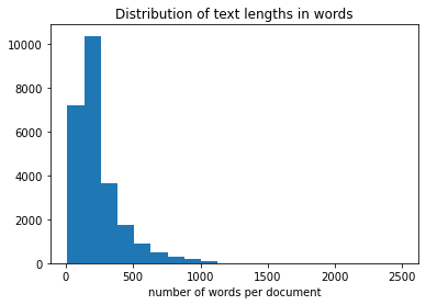
Next the distribution of review-lengths (words per review) is calculated:
textlenghtsTrain=[len(t) for t in X_train]
from matplotlib import pyplot as plt
plt.hist(textlenghtsTrain,bins=20)
plt.title("Distribution of text lengths in words")
plt.xlabel("number of words per document")
plt.show()
8.4.2. Preparing Text Sequences and Labels
All sequences must be padded to unique length of MAX_SEQUENCE_LENGTH. This means, that longer sequences are cut and shorter sequences are filled with zeros. For this Keras provides the pad_sequences()-function.
X_train = pad_sequences(X_train, maxlen=MAX_SEQUENCE_LENGTH)
X_test = pad_sequences(X_test, maxlen=MAX_SEQUENCE_LENGTH)
Moreover, all class-labels must be represented in one-hot-encoded form:
y_train = to_categorical(np.asarray(y_train))
y_test = to_categorical(np.asarray(y_test))
print('Shape of Training Data Input:', X_train.shape)
print('Shape of Training Data Labels:', y_train.shape)
Shape of Training Data Input: (25000, 500)
Shape of Training Data Labels: (25000, 2)
print('Number of positive and negative reviews in training and validation set ')
print (y_train.sum(axis=0))
print (y_test.sum(axis=0))
Number of positive and negative reviews in training and validation set
[12500. 12500.]
[12500. 12500.]
8.4.3. CNN with 2 Convolutional Layers
The first network architecture consists of
an embedding layer. This layer takes sequences of integers and learns word-embeddings. The sequences of word-embeddings are then passed to the first convolutional layer
two 1D-convolutional layers with different number of filters and different filter-sizes
two Max-Pooling layers to reduce the number of neurons, required in the following layers
a MLP classifier with one hidden layer and the output layer
8.4.3.1. Prepare Embedding Matrix and -Layer
embedding_layer = Embedding(MAX_NB_WORDS,
                            EMBEDDING_DIM,
                            #weights=[embedding_matrix],
                            input_length=MAX_SEQUENCE_LENGTH,
                            trainable=True)
8.4.3.2. Define CNN architecture
sequence_input = Input(shape=(MAX_SEQUENCE_LENGTH,), dtype='int32')
embedded_sequences = embedding_layer(sequence_input)
l_cov1= Conv1D(32, 5, activation='relu')(embedded_sequences)
l_pool1 = MaxPooling1D(2)(l_cov1)
l_cov2 = Conv1D(64, 3, activation='relu')(l_pool1)
l_pool2 = MaxPooling1D(5)(l_cov2)
l_flat = Flatten()(l_pool2)
l_dense = Dense(64, activation='relu')(l_flat)
preds = Dense(2, activation='softmax')(l_dense)
model = Model(sequence_input, preds)
8.4.3.3. Train Network
model.compile(loss='categorical_crossentropy',
              optimizer='rmsprop',
              metrics=['categorical_accuracy'])
model.summary()
Model: "model"
_________________________________________________________________
Layer (type)                 Output Shape              Param #
=================================================================
input_1 (InputLayer)         [(None, 500)]             0
_________________________________________________________________
embedding (Embedding)        (None, 500, 100)          1000000
_________________________________________________________________
conv1d (Conv1D)              (None, 496, 32)           16032
_________________________________________________________________
max_pooling1d (MaxPooling1D) (None, 248, 32)           0
_________________________________________________________________
conv1d_1 (Conv1D)            (None, 246, 64)           6208
_________________________________________________________________
max_pooling1d_1 (MaxPooling1 (None, 49, 64)            0
_________________________________________________________________
flatten (Flatten)            (None, 3136)              0
_________________________________________________________________
dense (Dense)                (None, 64)                200768
_________________________________________________________________
dense_1 (Dense)              (None, 2)                 130
=================================================================
Total params: 1,223,138
Trainable params: 1,223,138
Non-trainable params: 0
_________________________________________________________________
print("model fitting - simplified convolutional neural network")
history=model.fit(X_train, y_train, validation_data=(X_test, y_test),epochs=6, verbose=False, batch_size=128)
model fitting - simplified convolutional neural network
%matplotlib inline
from matplotlib import pyplot as plt
acc = history.history['categorical_accuracy']
val_acc = history.history['val_categorical_accuracy']
max_val_acc=np.max(val_acc)

epochs = range(1, len(acc) + 1)

plt.figure(figsize=(8,6))

plt.plot(epochs, acc, 'bo', label='Training accuracy')
plt.plot(epochs, val_acc, 'b', label='Validation accuracy')
plt.title('Training and validation accuracy')
plt.grid(True)
plt.legend()
plt.show()
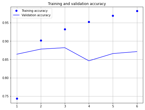
model.evaluate(X_test,y_test)
782/782 [==============================] - 4s 4ms/step - loss: 0.4747 - categorical_accuracy: 0.8711
[0.4746704399585724, 0.8711199760437012]
As shown above, after 6 epochs of training the cross-entropy-loss is 0.475 and the accuracy is 87.11%. However, it seems that the accuracy-value after 3 epochs has been higher, than the accuracy after 6 epochs. This indicates overfitting due to too long learning.
8.4.4. CNN with different filter sizes in one layer
In Y. Kim; Convolutional Neural Networks for Sentence Classification a CNN with different filter-sizes in one layer has been proposed. This CNN is implemented below:
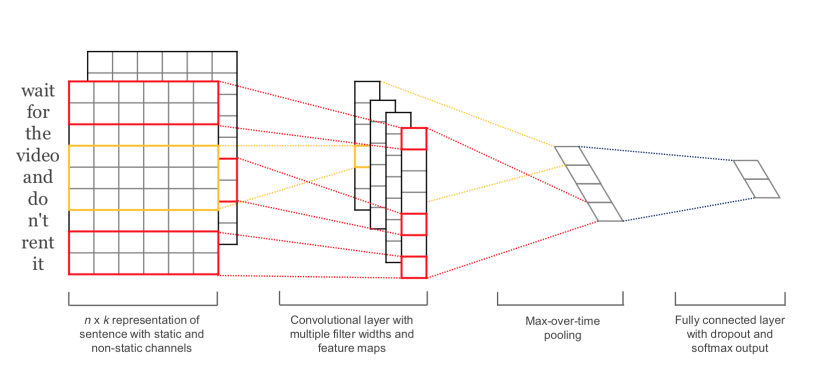
Source: Y. Kim; Convolutional Neural Networks for Sentence Classification
8.4.4.1. Prepare Embedding Matrix and -Layer
embedding_layer = Embedding(MAX_NB_WORDS,
                            EMBEDDING_DIM,
                            #weights=[embedding_matrix],
                            input_length=MAX_SEQUENCE_LENGTH,
                            trainable=True)
8.4.4.2. Define Architecture
convs = []
filter_sizes = [3,4,5]

sequence_input = Input(shape=(MAX_SEQUENCE_LENGTH,), dtype='int32')
embedded_sequences = embedding_layer(sequence_input)

for fsz in filter_sizes:
    l_conv = Conv1D(filters=32,kernel_size=fsz,activation='relu')(embedded_sequences)
    l_pool = MaxPooling1D(4)(l_conv)
    convs.append(l_pool)

l_merge = Concatenate(axis=1)(convs)
l_cov1= Conv1D(64, 5, activation='relu')(l_merge)
l_pool1 = GlobalMaxPool1D()(l_cov1)
#l_cov2 = Conv1D(128, 5, activation='relu')(l_pool1)
#l_pool2 = MaxPooling1D(30)(l_cov2)
l_flat = Flatten()(l_pool1)
l_dense = Dense(64, activation='relu')(l_flat)
preds = Dense(2, activation='softmax')(l_dense)

model = Model(sequence_input, preds)
model.summary()
Model: "functional_7"
__________________________________________________________________________________________________
Layer (type)                    Output Shape         Param #     Connected to
==================================================================================================
input_4 (InputLayer)            [(None, 500)]        0
__________________________________________________________________________________________________
embedding_2 (Embedding)         (None, 500, 100)     1000000     input_4[0][0]
__________________________________________________________________________________________________
conv1d_6 (Conv1D)               (None, 498, 32)      9632        embedding_2[0][0]
__________________________________________________________________________________________________
conv1d_7 (Conv1D)               (None, 497, 32)      12832       embedding_2[0][0]
__________________________________________________________________________________________________
conv1d_8 (Conv1D)               (None, 496, 32)      16032       embedding_2[0][0]
__________________________________________________________________________________________________
max_pooling1d_6 (MaxPooling1D)  (None, 124, 32)      0           conv1d_6[0][0]
__________________________________________________________________________________________________
max_pooling1d_7 (MaxPooling1D)  (None, 124, 32)      0           conv1d_7[0][0]
__________________________________________________________________________________________________
max_pooling1d_8 (MaxPooling1D)  (None, 124, 32)      0           conv1d_8[0][0]
__________________________________________________________________________________________________
concatenate (Concatenate)       (None, 372, 32)      0           max_pooling1d_6[0][0]
                                                                 max_pooling1d_7[0][0]
                                                                 max_pooling1d_8[0][0]
__________________________________________________________________________________________________
conv1d_9 (Conv1D)               (None, 368, 64)      10304       concatenate[0][0]
__________________________________________________________________________________________________
global_max_pooling1d (GlobalMax (None, 64)           0           conv1d_9[0][0]
__________________________________________________________________________________________________
flatten_3 (Flatten)             (None, 64)           0           global_max_pooling1d[0][0]
__________________________________________________________________________________________________
dense_6 (Dense)                 (None, 64)           4160        flatten_3[0][0]
__________________________________________________________________________________________________
dense_7 (Dense)                 (None, 2)            130         dense_6[0][0]
==================================================================================================
Total params: 1,053,090
Trainable params: 1,053,090
Non-trainable params: 0
__________________________________________________________________________________________________
8.4.4.3. Train Network
model.compile(loss='categorical_crossentropy',
              optimizer='rmsprop',
              metrics=['categorical_accuracy'])
print("model fitting - more complex convolutional neural network")
history=model.fit(X_train, y_train, validation_data=(X_test, y_test),epochs=8, batch_size=128)
model fitting - more complex convolutional neural network
Epoch 1/8
196/196 [==============================] - 48s 245ms/step - loss: 0.4927 - categorical_accuracy: 0.7368 - val_loss: 0.4006 - val_categorical_accuracy: 0.8133
Epoch 2/8
196/196 [==============================] - 51s 263ms/step - loss: 0.2560 - categorical_accuracy: 0.8971 - val_loss: 0.3341 - val_categorical_accuracy: 0.8614
Epoch 3/8
196/196 [==============================] - 49s 251ms/step - loss: 0.1860 - categorical_accuracy: 0.9280 - val_loss: 0.2924 - val_categorical_accuracy: 0.8814
Epoch 4/8
196/196 [==============================] - 48s 245ms/step - loss: 0.1286 - categorical_accuracy: 0.9536 - val_loss: 0.4191 - val_categorical_accuracy: 0.8469
Epoch 5/8
196/196 [==============================] - 47s 241ms/step - loss: 0.0829 - categorical_accuracy: 0.9731 - val_loss: 0.3308 - val_categorical_accuracy: 0.8890
Epoch 6/8
196/196 [==============================] - 47s 241ms/step - loss: 0.0506 - categorical_accuracy: 0.9840 - val_loss: 0.3952 - val_categorical_accuracy: 0.8771
Epoch 7/8
196/196 [==============================] - 47s 241ms/step - loss: 0.0266 - categorical_accuracy: 0.9923 - val_loss: 0.4222 - val_categorical_accuracy: 0.8806
Epoch 8/8
196/196 [==============================] - 47s 241ms/step - loss: 0.0152 - categorical_accuracy: 0.9954 - val_loss: 0.4665 - val_categorical_accuracy: 0.8847
acc = history.history['categorical_accuracy']
val_acc = history.history['val_categorical_accuracy']
max_val_acc=np.max(val_acc)

epochs = range(1, len(acc) + 1)

plt.figure(figsize=(8,6))

plt.plot(epochs, acc, 'bo', label='Training accuracy')
plt.plot(epochs, val_acc, 'b', label='Validation accuracy')
plt.title('Training and validation accuracy')
plt.grid(True)
plt.legend()
plt.show()
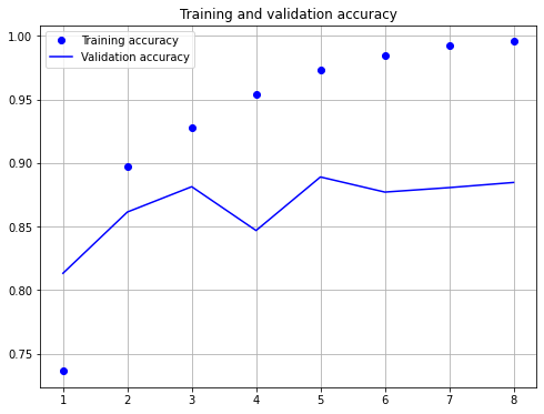
model.evaluate(X_test,y_test)
  1/782 [..............................] - ETA: 0s - loss: 0.4959 - categorical_accuracy: 0.8750WARNING:tensorflow:Callbacks method `on_test_batch_end` is slow compared to the batch time (batch time: 0.0098s vs `on_test_batch_end` time: 0.0219s). Check your callbacks.
782/782 [==============================] - 6s 7ms/step - loss: 0.4665 - categorical_accuracy: 0.8847
[0.46650105714797974, 0.8846799731254578]
As shown above, after 8 epochs of training the cross-entropy-loss is 0.467 and the accuracy is 88.47%.
8.4.5. LSTM
from tensorflow.keras.layers import LSTM, Bidirectional
embedding_layer = Embedding(MAX_NB_WORDS,
                            EMBEDDING_DIM,
                            #weights=[embedding_matrix],
                            input_length=MAX_SEQUENCE_LENGTH,
                            trainable=True)
sequence_input = Input(shape=(MAX_SEQUENCE_LENGTH,), dtype='int32')
embedded_sequences = embedding_layer(sequence_input)
l_lstm = Bidirectional(LSTM(64))(embedded_sequences)
preds = Dense(2, activation='softmax')(l_lstm)
model = Model(sequence_input, preds)
model.summary()
Model: "functional_3"
_________________________________________________________________
Layer (type)                 Output Shape              Param #
=================================================================
input_2 (InputLayer)         [(None, 500)]             0
_________________________________________________________________
embedding_1 (Embedding)      (None, 500, 100)          1000000
_________________________________________________________________
bidirectional_1 (Bidirection (None, 128)               84480
_________________________________________________________________
dense_1 (Dense)              (None, 2)                 258
=================================================================
Total params: 1,084,738
Trainable params: 1,084,738
Non-trainable params: 0
_________________________________________________________________
model.compile(loss='categorical_crossentropy',
              optimizer='rmsprop',
              metrics=['categorical_accuracy'])

print("model fitting - Bidirectional LSTM")
model fitting - Bidirectional LSTM
history=model.fit(X_train, y_train, validation_data=(X_test, y_test),epochs=6, batch_size=128)
Epoch 1/6
196/196 [==============================] - 109s 559ms/step - loss: 0.4442 - categorical_accuracy: 0.7918 - val_loss: 0.5594 - val_categorical_accuracy: 0.7815
Epoch 2/6
196/196 [==============================] - 107s 546ms/step - loss: 0.2801 - categorical_accuracy: 0.8875 - val_loss: 0.2959 - val_categorical_accuracy: 0.8790
Epoch 3/6
196/196 [==============================] - 111s 565ms/step - loss: 0.2310 - categorical_accuracy: 0.9109 - val_loss: 0.3848 - val_categorical_accuracy: 0.8536
Epoch 4/6
196/196 [==============================] - 110s 562ms/step - loss: 0.2017 - categorical_accuracy: 0.9248 - val_loss: 0.3087 - val_categorical_accuracy: 0.8729
Epoch 5/6
196/196 [==============================] - 107s 547ms/step - loss: 0.1767 - categorical_accuracy: 0.9362 - val_loss: 0.3703 - val_categorical_accuracy: 0.8671
Epoch 6/6
196/196 [==============================] - 105s 538ms/step - loss: 0.1551 - categorical_accuracy: 0.9435 - val_loss: 0.4671 - val_categorical_accuracy: 0.8670
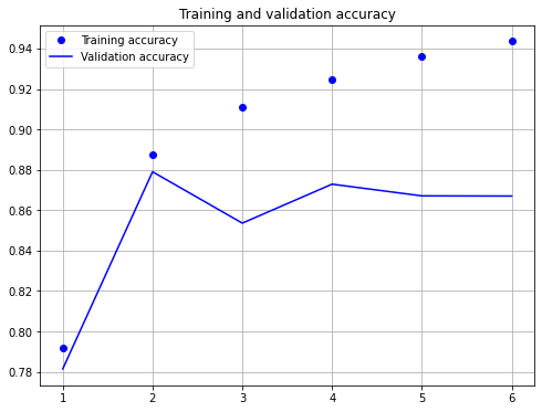
acc = history.history['categorical_accuracy']
val_acc = history.history['val_categorical_accuracy']
max_val_acc=np.max(val_acc)

epochs = range(1, len(acc) + 1)

plt.figure(figsize=(8,6))

plt.plot(epochs, acc, 'bo', label='Training accuracy')
plt.plot(epochs, val_acc, 'b', label='Validation accuracy')
plt.title('Training and validation accuracy')
plt.grid(True)
plt.legend()
plt.show()
model.evaluate(X_test,y_test)
782/782 [==============================] - 24s 31ms/step - loss: 0.4671 - categorical_accuracy: 0.8670
[0.467098593711853, 0.8669999837875366]
As shown above, after 6 epochs of training the cross-entropy-loss is 0.467 and the accuracy is 86.7%. However, it seems that the accuracy-value after 2 epochs has been higher, than the accuracy after 6 epochs. This indicates overfitting due to too long learning.
8.4.6. Bidirectional LSTM architecture with Attention
8.4.6.1. Define Custom Attention Layer
Since Keras does not provide an attention-layer, we have to implement this type on our own. The implementation below corresponds to the attention-concept as introduced in Bahdanau et al: Neural Machine Translation by Jointly Learning to Align and Translate.
The general concept of writing custom Keras layers is described in the corresponding Keras documentation.
Any custom layer class inherits from the layer-class and must implement three methods:
build(input_shape): this is where you will define your weights. This method must setself.built = True, which can be done by callingsuper([Layer], self).build().call(x): this is where the layer’s logic lives. Unless you want your layer to support masking, you only have to care about the first argument passed to call: the input tensor.compute_output_shape(input_shape): in case your layer modifies the shape of its input, you should specify here the shape transformation logic. This allows Keras to do automatic shape inference.
from tensorflow.keras import regularizers, initializers,constraints
from tensorflow.keras.layers import Layer


class Attention(Layer):
    def __init__(self, step_dim,
                 W_regularizer=None, b_regularizer=None,
                 W_constraint=None, b_constraint=None,
                 bias=True, **kwargs):
        self.supports_masking = True
        self.init = initializers.get('glorot_uniform')

        self.W_regularizer = regularizers.get(W_regularizer)
        self.b_regularizer = regularizers.get(b_regularizer)

        self.W_constraint = constraints.get(W_constraint)
        self.b_constraint = constraints.get(b_constraint)

        self.bias = bias
        self.step_dim = step_dim
        self.features_dim = 0
        super(Attention, self).__init__(**kwargs)

    def build(self, input_shape):
        assert len(input_shape) == 3

        self.W = self.add_weight(shape=(input_shape[-1],),
                                 initializer=self.init,
                                 name='{}_W'.format(self.name),
                                 regularizer=self.W_regularizer,
                                 constraint=self.W_constraint)
        self.features_dim = input_shape[-1]

        if self.bias:
            self.b = self.add_weight(shape=(input_shape[1],),
                                     initializer='zero',
                                     #name='{}_b'.format(self.name),
                                     regularizer=self.b_regularizer,
                                     constraint=self.b_constraint)
        else:
            self.b = None

        self.built = True

    def compute_mask(self, input, input_mask=None):
        return None

    def call(self, x, mask=None):
        features_dim = self.features_dim
        step_dim = self.step_dim

        eij = K.reshape(K.dot(K.reshape(x, (-1, features_dim)),
                        K.reshape(self.W, (features_dim, 1))), (-1, step_dim))

        if self.bias:
            eij += self.b

        eij = K.tanh(eij)

        a = K.exp(eij)

        if mask is not None:
            a *= K.cast(mask, K.floatx())

        a /= K.cast(K.sum(a, axis=1, keepdims=True) + K.epsilon(), K.floatx())

        a = K.expand_dims(a)
        weighted_input = x * a
        return K.sum(weighted_input, axis=1)

    def compute_output_shape(self, input_shape):
        return input_shape[0],  self.features_dim
embedding_layer = Embedding(MAX_NB_WORDS,
                            EMBEDDING_DIM,
                            #weights=[embedding_matrix],
                            input_length=MAX_SEQUENCE_LENGTH,
                            trainable=True)
sequence_input = Input(shape=(MAX_SEQUENCE_LENGTH,), dtype='int32')
embedded_sequences = embedding_layer(sequence_input)
l_gru = Bidirectional(LSTM(64, return_sequences=True))(embedded_sequences)
l_att = Attention(MAX_SEQUENCE_LENGTH)(l_gru)
preds = Dense(2, activation='softmax')(l_att)
model = Model(sequence_input, preds)
model.summary()
Model: "functional_5"
_________________________________________________________________
Layer (type)                 Output Shape              Param #
=================================================================
input_13 (InputLayer)        [(None, 500)]             0
_________________________________________________________________
embedding_11 (Embedding)     (None, 500, 100)          1000000
_________________________________________________________________
bidirectional_11 (Bidirectio (None, 500, 128)          84480
_________________________________________________________________
attention_8 (Attention)      (None, 128)               628
_________________________________________________________________
dense_2 (Dense)              (None, 2)                 258
=================================================================
Total params: 1,085,366
Trainable params: 1,085,366
Non-trainable params: 0
_________________________________________________________________
model.compile(loss='categorical_crossentropy',
              optimizer='rmsprop',
              metrics=['categorical_accuracy'])
history=model.fit(X_train, y_train, validation_data=(X_test, y_test),epochs=6, batch_size=128)
Epoch 1/6
196/196 [==============================] - 126s 643ms/step - loss: 0.4488 - categorical_accuracy: 0.7836 - val_loss: 0.3027 - val_categorical_accuracy: 0.8777
Epoch 2/6
196/196 [==============================] - 125s 638ms/step - loss: 0.2596 - categorical_accuracy: 0.8984 - val_loss: 0.3228 - val_categorical_accuracy: 0.8691
Epoch 3/6
196/196 [==============================] - 126s 640ms/step - loss: 0.2071 - categorical_accuracy: 0.9197 - val_loss: 0.6833 - val_categorical_accuracy: 0.7630
Epoch 4/6
196/196 [==============================] - 123s 630ms/step - loss: 0.1791 - categorical_accuracy: 0.9323 - val_loss: 0.2992 - val_categorical_accuracy: 0.8779
Epoch 5/6
196/196 [==============================] - 128s 654ms/step - loss: 0.1553 - categorical_accuracy: 0.9417 - val_loss: 0.3247 - val_categorical_accuracy: 0.8788
Epoch 6/6
196/196 [==============================] - 130s 666ms/step - loss: 0.1335 - categorical_accuracy: 0.9509 - val_loss: 0.3339 - val_categorical_accuracy: 0.8695
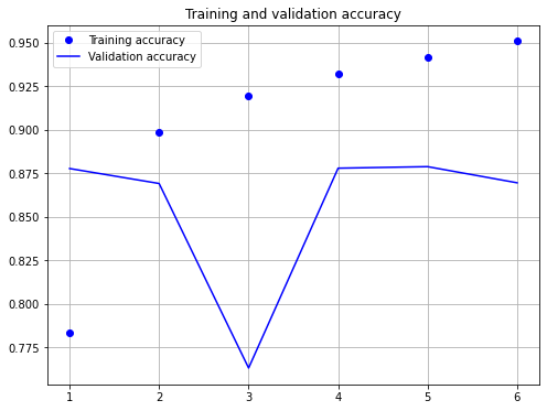
acc = history.history['categorical_accuracy']
val_acc = history.history['val_categorical_accuracy']
max_val_acc=np.max(val_acc)

epochs = range(1, len(acc) + 1)

plt.figure(figsize=(8,6))

plt.plot(epochs, acc, 'bo', label='Training accuracy')
plt.plot(epochs, val_acc, 'b', label='Validation accuracy')
plt.title('Training and validation accuracy')
plt.grid(True)
plt.legend()
plt.show()
model.evaluate(X_test,y_test)
782/782 [==============================] - 29s 37ms/step - loss: 0.3339 - categorical_accuracy: 0.8695
[0.33391639590263367, 0.8695200085639954]
Again, the achieved accuracy is in the same range as for the other architectures. None of the architectures has been optimized, e.g. through hyperparameter-tuning. However, the goal of this notebook is not the determination of an optimal model, but the demonstration of how modern neural network architectures can be implemented for text-classification.