
5.1. Vector Space Model
Vector Space Models map arbitrary inputs to numeric vectors of fixed length. For a given task, you are free to define a set of \(N\) relevant features, which can be extracted from the input. Each of the \(N\)-feature extraction functions returns how often the corresponding feature appears in the input. Each component of the vector-representation belongs to one feature and the value at this component is the count of this feature in the input.
Example: Vector Space Model in General
Assume that your task is to classify texts into the classes poetry and scientific paper. The classifier shall be learned by a Machine Learning Algorithm which requires fixed-length numeric vectors at it’s input. You think about relevant features and come to the conclusion, that
the average length of sentences (in words)
the number of proper names
the number of adjectives
may be relevant features. Then all input-texts, independent of their length can be mapped to vectors of length \(N=3\), whose components are the frequencies of this features in the text. E.g. the text
Mary loves the kind and handsome little boy. His name is Peter and he lived next door to Mary's jealous friend Anne.
maps into the vector
5.1.1. Bag-of-Word Model
In the general case the vector space model implies a vector, whose components are the frequencies of pre-defined features in the given input. In the special case of text (=documents), a vector space model is applied, where the features are defined to be all words of the vocabulary \(V\). I.e. each component in the resulting vector corresponds to a word \(w \in V\) and the value of the component is the frequency of this word in the given document. This vector space model for texts is the so called Bag of Words (BoW) model and the frequency of a word in a given document is denoted term-frequency. Accordingly a set of documents is modelled by a Bag of Words matrix, whose rows belong to documents and whose columns belong to words.
Example: Bag of Word matrix
Assume, that the given playground-corpus contains only two documents
Document 1: not all kids stay at home
Document 2: all boys and girls stay not at home
The BoW model of these documents is then
all |
and |
at |
boys |
girls |
home |
kids |
not |
stay |
|
|---|---|---|---|---|---|---|---|---|---|
Document 1 |
1 |
0 |
1 |
0 |
0 |
1 |
1 |
1 |
1 |
Document 2 |
1 |
1 |
1 |
1 |
1 |
1 |
0 |
1 |
1 |
In this example the words in the matrix have been alphabetically ordered. This is not necessary.
5.1.2. Bag-of-Word Variants
The entries of the BoW-matrix, as introduced above, are the term-frequencies. I.e. the entry in row \(i\), column \(j\), \(tf(i,j)\) determines how often the term (word) of column \(j\), appears in document \(i\).
Another option is the binary BoW. Here, the binary entry in row \(i\), column \(j\) just indicates if term \(j\) appears in document \(i\). The entry has value 1 if the term appears at least once, otherwise it is 0.
TF-IDF BoW: The drawback of using term-frequency \(tf(i,j)\) as matrix entries is that all terms are weighted similarly, in particular rare words such as words with a strong semantic focus are weighted in the same way as very frequent words, such as articles. TF-IDF is a weighted term frequency (TF). The weights are the inverse document frequencies (IDF). Actually, there are different definitions for the calculation of TF-IDF. A common definition is
where \(tf(i,j)\) is the frequency of term \(j\) in document \(i\), \(N\) is the total number of documents and \(df_j\) is the number of documents, which contain term \(j\). For words, which occure in all documents
i.e. such words are disregarded in a BoW with TF-IDF entries. Otherwise, words with a very strong semantic focus usually appear in only a few documents. Then the small value of \(df_j\) yields a low IDF, i.e. the term-frequency of such a word is weighted strongly.
5.1.3. One-Hot-Encoding of Words
In the extreme case of documents, which contain only a single word, the corresponding tf-based BoW-vector, has only one component of value 1 (in the column, which belongs to this word), all other entries are zero. This is actually a common conventional numeric encoding of words, the so called One-Hot-Encoding.
Example: One-Hot-Encoding of words
Assume, that the entire Vocabular is
A possible One-Hot-Encoding of these words is then
all |
1 |
0 |
0 |
0 |
0 |
0 |
0 |
0 |
0 |
and |
0 |
1 |
0 |
0 |
0 |
0 |
0 |
0 |
0 |
at |
0 |
0 |
1 |
0 |
0 |
0 |
0 |
0 |
0 |
boys |
0 |
0 |
0 |
1 |
0 |
0 |
0 |
0 |
0 |
girls |
0 |
0 |
0 |
0 |
1 |
0 |
0 |
0 |
0 |
home |
0 |
0 |
0 |
0 |
0 |
1 |
0 |
0 |
0 |
kids |
0 |
0 |
0 |
0 |
0 |
0 |
1 |
0 |
0 |
not |
0 |
0 |
0 |
0 |
0 |
0 |
0 |
1 |
0 |
stay |
0 |
0 |
0 |
0 |
0 |
0 |
0 |
0 |
1 |
5.1.4. BoW-based document similarity
Numeric vector presentation of documents are not only required for Machine-Learning based NLP tasks. Another important application category is Information Retrieval (IR). Information Retrieval deals with algorithms and models for searching information in large document collections. Web-search like www.google.com is only one example for IR. In such document-search applications the user defines a query, usually in terms of one or more words. The task of the IR system is then to
return relevant documents, which match the query
rank the returned documents, such that the most important is at the top of the search-result
Challenges in this context are:
How to deduce what the user actually wants, given only a few query-words?
How to calculate the relevance of a document with respect to the query words?
Question 1 will be addressed later further below, when Distributional Semantic Models, in particular Word Embeddings are introduced. The second question will be answered now.
The conventional approach for document search is to
model all documents in the index as numerical vectors, e.g. by BoW
model the query as a numerical vector in the same way as the documents are modelled
determine the most relevant documents by just determining the document-vectors, which have the smallest distance to the query-vector.
This means that the question on relevance is solved by determining nearest vectors in a vector space. An example is given below. Here we assume, that there are only 3 documents in the index and there are only 4 different words, occuring in these documents. Document 2, for example, contains word 1 with a frequency of 4 and word 2 with a frequency of 5. The query consists of word 1 and word 2. The BoW-matrix and the attached query-vector are:
word 1 |
word 2 |
word 3 |
word 4 |
|
|---|---|---|---|---|
document 1 |
1 |
1 |
1 |
1 |
document 2 |
4 |
5 |
0 |
0 |
document 3 |
0 |
0 |
1 |
1 |
Query |
1 |
1 |
0 |
0 |
Given these vector-representations, it is easy to determine the distances between each document and the query.
The obvious type of distance is the Euclidean Distance: For two vectors, \(\underline{a}=(a_1,\ldots,a_n)\) and \(\underline{b}=(b_1,\ldots,b_n)\), the Euclidean Distance is defined to be
Similarity and Distance are inverse to each other, i.e. the similarity between vectors increases with decreasing distance and vice versa. For each distance-measure a corresponding similarity-measure can be defined. E.g. the Euclidean-distance-based similarity measure is
Now let’s determine the Euclidean distance between the query and the 3 documents in the example abover:
Euclidean distance between query and document 1:
Euclidean distance between query and document 2:
Euclidean distance between query and document 3:
Comparing these 3 distances, one can conclude, that document 1 has the smallest distance (and the highest similarity) to the query and is therefore the best match.
Is this what we expect?
No! Document 2 contains the query words not only once but with a much higher frequency. One would expect, that this stronger prevalence of the query words implies that Document 2 is more relevant.
So what went wrong?
The answer is, that the Euclidean Distance is just the wrong distance-measure for this type of application. In a query each word is contained only once. Therefore, Euclidean-distance penalizes longer documents with more words.
The solution to this problem is
either normalize all vectors - document vectors and query-vector - to unique length,
or apply another distance measure
The standard similarity-measure for BoW vectors is the Cosine Similarity \(s_C(\underline{a},\underline{b})\), which is calculated as follows:
From the cosine-similarity measure the cosine-distance can be calculated as follows:
For the query-example above, the Cosine-Similarities are:
Cosine Similarity between query and document 2:
Cosine Similarity between query and document 2:
Cosine Similarity between query and document 3:
These calculated similarities match our subjective expectation: The similarity between document 3 and query \(q\) is 0 (the lowest possible value), since they have no word in common. The similarity between document 2 and the query q is close to the maximum similarity-value of 1, since both query-words appear with a high frequency in this document.
Another similarity measure is the Pearson Correlation \(s_P(\underline{a},\underline{b})\). The Pearson correlation coefficient measures linearity, i.e. its maximum value of \(s_P(\underline{a},\underline{b})=1\) is obtained, if there is a linear correlation between the two vectors. Pearson correlation is calculated as follows:
where
and
and
\(\overline{a}\) is the mean over the components in \(\underline{a}\) and \(\overline{b}\) is the mean over the components in \(\underline{b}\).
The corresponding distance measure is:
There exists much more distance- and similarity-measures, see e.g. scipy.spatial.distance or Distance Measures in Data Science.
5.1.5. BoW Drawbacks
BoW representation of documents and the One-Hot-Encoding of single words, as described above, are methods to map words and documents to numeric vectors, which can be applied as input for arbitrary Machine Learning algorithms. Hovever, these representations suffer from crucial drawbacks:
The vectors are usually very long - there length is given by the number of words in the vocabulary. Moreover, the vectors are quite sparse, since the set of words appearing in one document is usually only a very small part of the set of all words in the vocabulary.
Semantic relations between words are not modelled. This means that in this model there is no information about the fact that word car is more related to word vehicle than to word lake.
In the BoW-model of documents word order is totally ignored. E.g. the model can not distinguish if word not appeared immediately before word good or before word bad.
All of these drawbacks can be solved by
applying Distributional Semantic Models for caluclating better vector-representations of words
pass these vector-representations of words to the input of neural network architectures such as Recurrent Neural Networks (RNNs), Convolutional Neural Networks (CNNs) or Transformers (see later chapters of this lecture).
5.2. Distributional Semantic Models
The linguistic theory of distributional semantics is based on the hypothesis, that words, which occur in similar contexts, have similar meaning. J.R. Firth formulated this assumption in his famous sentence [Fir57]:
You shall know a word by the company it keeps
Since computers can easily determine the co-occurrence statistics of words in large corpora the theory of distributional semantics provides a promising opportunity to automatically learn semantic relations. The learned semantic representations are called Distributional Semantic Models (DSM). They represent each word as a numerical vector, such that words, which appear frequently in similar contexts, are represented by similar vectors. In the figure below the arrow represents the DSM. Since there are many different DSMs there are many different approaches to implement this transformation from the hypothesis of distributional semantics to the word-vector-space.

The field of DSMs can be categorized into the classes count-based models and prediction-based models. Recently, considerable attention has been focused on the question which of these classes is superior [PSM14].
5.2.1. Count-based DSM
DSMs map words to numeric vectors, such that semantically related words, i.e. words which appear frequently in a similar context, have similar numeric vectors. The first question which arises from this definition is What is context? In all DSMs, introduced in this lecture, the context of a target word \(w\) is considered to be the sequence of \(L\) previous and \(L\) following words, where the context-length \(L\) is a parameter.
I.e. in the word-sequence
the words \(w_{i-L},\ldots,w_{i-1},w_{i+1},\ldots,w_{i+L}\) constitute the context of target word \(w_i\) and
is the corresponding set of word-context-pairs w.r.t. target word \(w_i\).
The most common numeric vector representation of count-based DSMs can be derived from the Word-Co-Occurence matrix. In this matrix each row belongs to a target-word and each column belongs to a context word. Hence, the matrix has usually \(\mid V \mid\) rows and the same amount of columns1. In this matrix the entry in row \(i\), column \(j\) is the number of times context word \(c_j\) appears in the context of target word \(w_i\). This frequency is denoted by \(\#(w_i,c_j)\). The structure of such a word-co-occurence matrix is given below:

In order to determine this matrix a large corpus of contigous text is required. Then for all target-context pairs the corresponding count \(\#(w_i,c_j)\) must be determined. Once the matrix is complete the numeric vector representation of word \(w_i\) is just the i.th row in this matrix!.
Example: Word-Co-Occurence Matrix
Assume that the (unrealistically small) corpus is
K = The dusty road ends nowhere. The dusty track ends there.
For a (unrealistically small) context length of \(L=2\) the word-co-occurence matrix is:

With this matrix, the numeric vector representation of word road is:
and the vector for word track is:
As can be seen, these two vectors are quite similar. The reason for this similarity is that both words appear in similar contexts. Hence we assume that they are semantically correlated.
With respect to the drawbacks of BoW-vectors as mentioned in subsection BoW Drawbacks, the count-based DSM-vectors provide the important advantage of modelling semantic relations between words: Pairs of semantically related words are closer to each other, than unrelated words. However, the count-based DSM vectors, as introduced so far, still suffer from the drawback of long and sparse vectors. This drawback can be eliminated by applying a dimensionality reduction such as Principal Component Analysis (PCA) or Singular Value Decomposition (SVD), which are introduced later on in this lecture.
5.2.1.1. Variants of count-based DSMs
Count-based DSMs differ in the following parameters:
Context-Modelling: In any case the rows in the word-context matrix are the vector-representation of the corresponding word, i.e. each row uniquely corresponds to a word. The columns describe the context, but different types of context can be considered, e.g. the context can be defined by the previous words or the previous and following words. Moreover, the window-size, which defines the number of surrounding words, which are considered to be within the context is an important parameter.
Preprocessing: Different types of preprocessing, e.g. stop-word-filtering, high-frequency cut-off, normalisation, lemmatization can be applied to the given corpus. Different preprocessing techniques yield different word-context matrices.
Weighting Scheme: The entries \(w_{ij}\) in the word-context matrix somehow measure the association between target-word \(i\) and context-word \(j\). In the most simple case \(w_{ij}\) is just the frequency of word \(j\) in the context of word \(i\). However, many different alternatives for defining the entries in the word-co-occuruence-matrix exist. For example
the conditional probability \(P(c_j|w_i)\), which is determined by
\[ P(c_j|w_i)=\frac{\#(w_i,c_j)}{\#(w_i)}, \]the pointwise mutual information (PMI) of \(w_i\) and \(c_j\)
\[ PMI(w_i,c_j)=\log_2 \frac{P(w_i,c_j)}{P(w_i)P(c_j)} = \log_2 \frac{\#(w_i,c_j) |D|}{\#(w_i) \#(c_j)}, \]where \(D\) is the training corpus and \(\mid D \mid\) is the number of words in this corpus,
the positive pointwise mutual information (PPMI):
\[ PPMI(w_i,c_j) = \max\left(PMI(w_i,c_j),0 \right). \]
Dimensionality Reduction: Depending on the definition of context the word vectors may be very sparse. Transforming these sparse vectors to a lower dimensional space yields a lower complexity, but may also yield better generalisation of the model. Different dimensionality reduction schemes such as PCA, SVD or autoencoder yield different word-vector spaces.
Size of word vectors: The size of the word vectors depend on context modelling, preprocessing and dimensionality reduction.
Similarity-/Distance-Measure. In count-based word-spaces different metrics to measure similarity between the word vectors can be applied, e.g. cosine-similarity or Hellinger distance. The performance of the word-space model strongly depends on the applied similarity measure.
5.2.2. Prediction-based DSM
In 2013 Mikolov et al. published their milestone-paper Efficient Estimation of Word Representations in Vector Space [MSC+13]. They proposed quite simple neural network architectures to efficiently create DSM word-embeddings: CBOW and Skipgram. These architectures are better known as Word2Vec. In both techniques neural networks are trained for a pseudo-task. After training, the network itself is usually not of interest. However, the learned weights in the input-layer constitute the word-embeddings, which can then be applied for a large field of NLP-tasks, e.g. document classification.
5.2.2.1. Continous Bag-Of-Words (CBOW)
The idea of CBOW is to predict the target word \(w_i\), given the \(N\) context-words \(w_{i-N/2},\ldots, w_{i-1}, \quad w_{i+1}, w_{i+N/2}\). In order to learn such a predictor a large but unlabeled corpus is required. The extraction of training-samples from a corpus is sketched in the picture below:
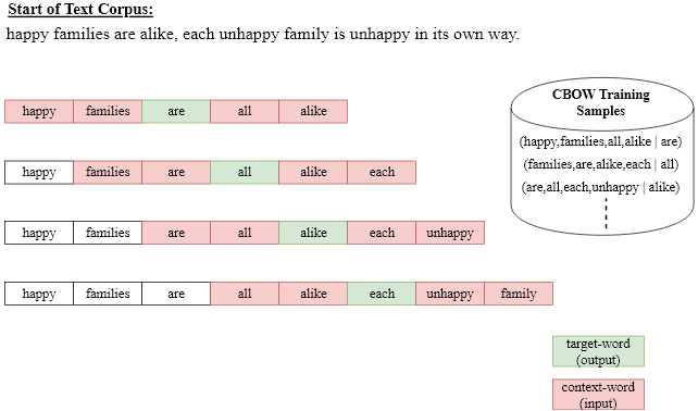
In this example a context length of \(N=4\) has been applied. The first training-element consists of
the \(N=4\) input-words (happy,families,all,alike)
the target word are.
In order to obtain the second training-sample the window of length \(N+1\) is just shifted by one to the right. The concrete architecture for CBOW is shown in the picture below. At the input the \(N\) context words are one-hot-encoded. The fully-connected Projection-layer maps the context words to a vector representation of the context. This vector representation is the input of a softmax-output-layer. The output-layer has as much neurons as there are words in the vocabulary \(V\). Each neurons uniquely corresponds to a word of the vocabulary and outputs an estimation of the probaility, that the word appears as target for the current context-words at the input.
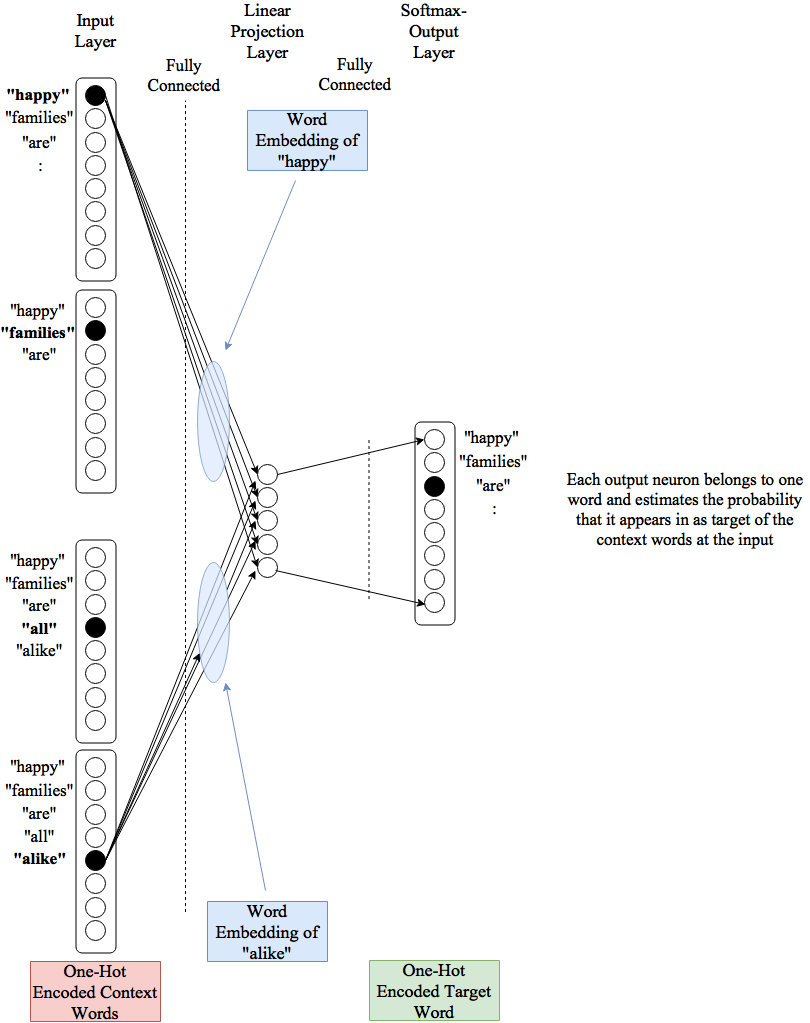
After training the CBOW-network the vector representation of word \(w\) are the weights from the one-hot encoded word \(w\) at the input of the network to the neurons in the projection-layer. I.e. the number of neurons in the projection layer define the length of the word-embedding.
5.2.2.2. Skip-Gram
Skip-Gram is similar to CBOW, but has a reversed prediction process: For a given target word at the input, the Skip-Gram model predicts words, which are likely in the context of this target word. Again, the context is defined by the \(N\) neighbouring words. The extraction of training-samples from a corpus is sketched in the picture below:
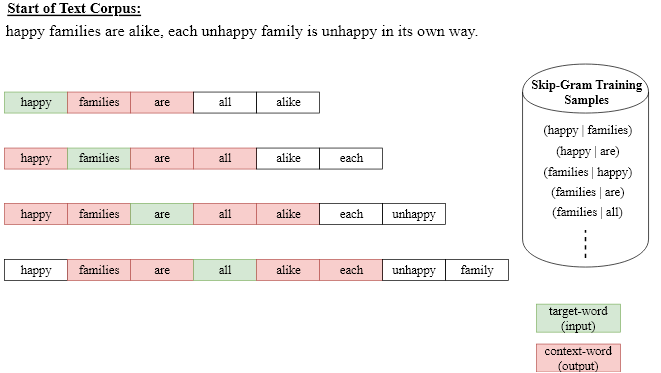
Again a context length of \(N=4\) has been applied. The first training-element consists of
the first target word (happy) as input to the network
the first context word (families) as network-output.
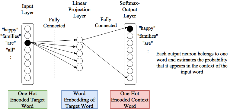
The concrete architecture for Skip-gram is shown in the picture below. At the input the target-word is one-hot-encoded. The fully-connected Projection-layer outputs the current vector representation of the target-word. This vector representation is the input of a softmax-output-layer. The output-layer has as much neurons as there are words in the vocabulary \(V\). Each neurons uniquely corresponds to a word of the vocabulary and outputs an estimation of the probaility, that the word appears in the context of the current target-word at the input.
5.2.2.3. GloVe
In light of the two different approaches of DSMs, count-based and prediction-based models, Pennington et al developed in [PSM14] an approach called Global Vectors, which claims to combine the advantages of both DSM types. The advantage of count-based models is that they capture global co-occurrence statistics. Prediction based models do not operate on the global co-occurence statistics, but scan context windows across the entire corpus. On the other hand prediction-based models demonstrated in many evaluations that they are capable to learn linguistic patterns as linear relationships between the word vectors, indicating a vector space structure, which reflects linguistic semantics.
GloVe integrates the advantages of both approaches by minimizing a loss function, which is a weighted least-square function, that contains the difference between the scalar-product of a word vector \(w_i\) and a context vector \(\tilde{w}_j\) and the logarithm of the word-cooccruence-matrix-entry \(\#(w_i,c_j)\) (see [PSM14] for more details).
5.2.2.4. FastText
Another word embedding model is fastText from Facebook, which was introduced in 2017 [BGJM16] 2. fastText is based on the Skipgram architecture, but instead using at the input the words itself, it applies character-sequences of length \(n\) (n-grams on character-level). For example for $n=3, the word fastText would be presented as the following set of character-level 3-grams:
The advantages of this approach over word embeddings, that work on word level.
The morphology of words is taken into account, which is especially important in languages with large vocabularies and many rare words - such as German.
Prefixes, suffixes and compound words can be better understood
for words, which appear not in the training, it is likely that sub-n-grams are available
5.2.3. DSM Downstream tasks
By applying DSM one can reliably determine for a given query word a set of semantically or syntactically related word by nearest-neighbour search in a vector space. In the picture below (Source: [CWB+11]) for some query words (in the topmost row of the table), the words, whose vectors are closest to the vector of the query-word are listed. For example, the word-vectors, which are closest to the vector of France are: Austria, Belgium, Germany, …

Moreover, as shown in the picture below (Source: [MSC+13]), also semantic relations between pairs of words can be determined, by subtracting one vector from the other. For example subtracting the vector for man from the vector of woman is another vector, which represents the female-male-relation. Adding this vector to the vector of king results in the vector of queen. Hence word embeddings can solve questions like men ist to woman as queen is to? 3.

The ability to model semantic similarity and semantic relations has made Word-Embedings an essential building block for many NLP applications (downstream tasks) [Bak18], e.g.
Noun Phrase Chunking
Named Entity Recognition (NER)
Sentiment Analysis: Determine sentiment in sentences and text
Syntax Parsing: Determine the syntax tree of a sentence
Semantic Role Labeling (SRL): see e.g. [JM09] for a definition of semantic roles
Negation Scope Detection
POS-Tagging
Text Classification
Metaphor Detection
Paraphrase Detection
Textual Entailment Detection: Determine if some a text-part is an entailment of another
Automatic Translation
All in all, since their breakthrough in 2013 ([MSC+13]), prediction based Word-Embeddings have revolutionized many NLP applications.
- 1
One may have different vocabularies for target-words (\(V_W\)) and context-words (\(V_C\)). However, often they coincide, i.e. \(V = V_W=V_C\).
- 2
Actually fastText has been introduced already in 2016, but not as a Word-Embedding, but as a text classifier. In 2017 it has been adapted as a word-embedding.
- 3
It has been shown that such relations can be determined by prediction-based DSMs, but not with conventional count-based DSMs.