
Bayesian Networks with pyAgrum
Contents
Bayesian Networks with pyAgrum#
Bayesian Networks (BNs) are class of Probabilistic Graphical Models that are capable to reason under uncertainty. They can be seen as a probabilistic expert system: the domain knowledge (business knowledge) is modeled as direct acyclic graph (DAG). The nodes of this DAG represent the random variables and the arcs between the nodes represent the probabilistic dependencies (correlation, causation or influence) between the variables. Morevoer, a conditional probability table (CPT) is associated with each node. It contains the conditional probability distribution of the node given its parents in the DAG.
In this section the famous Visit Asia1 Bayes Net shall be implemented in pyAgrum.
The asia data set contains the following variables:
D (dyspnoea), a two-level factor with levels yes and no.
T (tuberculosis), a two-level factor with levels yes and no.
L (lung cancer), a two-level factor with levels yes and no.
B (bronchitis), a two-level factor with levels yes and no.
A (visit to Asia), a two-level factor with levels yes and no.
S (smoking), a two-level factor with levels yes and no.
X (chest X-ray), a two-level factor with levels yes and no.
E (tuberculosis versus lung cancer/bronchitis), a two-level factor with levels yes and no.
Motivation:
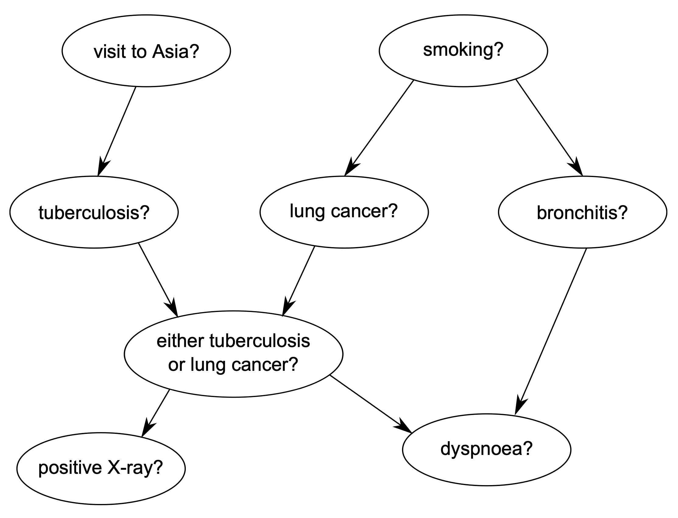
Shortness-of-breath (dyspnoea) may be due to tuberculosis, lung cancer or bronchitis, or none of them, or more than one of them. A recent visit to Asia increases the chances of tuberculosis, while smoking is known to be a risk factor for both lung cancer and bronchitis. The results of a single chest X-ray do not discriminate between lung cancer and tuberculosis, as neither does the presence or absence of dyspnoea.
The structure of the Bayesian Network is depicted below:
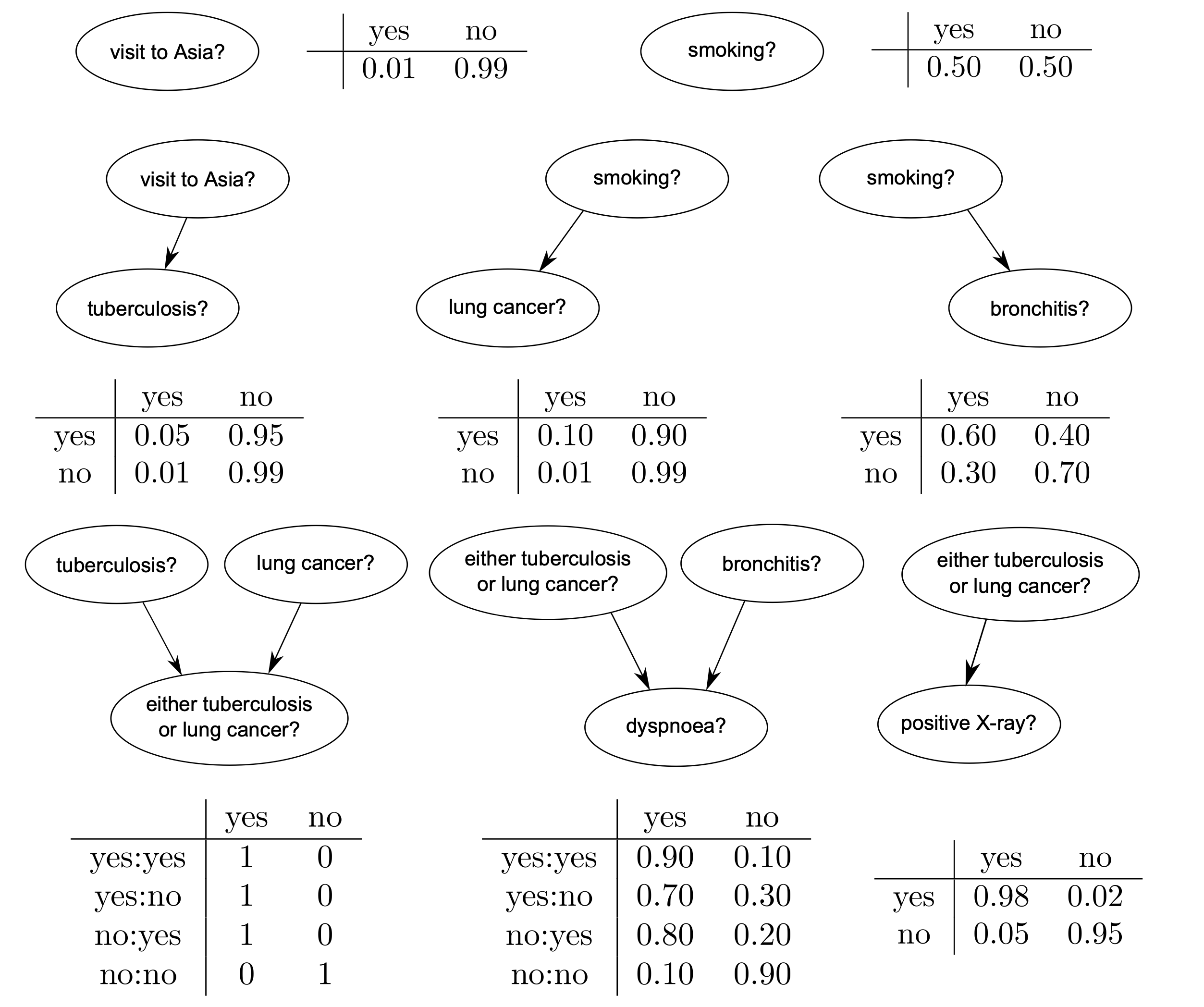
The Conditional Propability Tables (CPT) for each node are shown below:
from pylab import *
import matplotlib.pyplot as plt
import os
import pyAgrum as gum
Create the network topology#
The next line creates an empty BN network with a ‘name’ property.
bn=gum.BayesNet('Asia')
print(bn)
BN{nodes: 0, arcs: 0, domainSize: 1, dim: 0}
Create the variables#
pyAgrum provides 3 types of variables :
LabelizedVariableRangeVariableDiscretizedVariable
In this example LabelizedVariable, which is a variable whose domain is a finite set of labels.
In the code cell below a variable named A, with 2 values and described as visit to Asia? is created and added to the BN. The value returned is the id of the node in the graphical structure (the DAG). pyAgrum actually distinguishes the random variable (here the LabelizedVariable) from its node in the DAG: the latter is identified through a numeric id.
A=bn.add(gum.LabelizedVariable('A','visit to Asia?',2))
print(A)
0
S=bn.add(gum.LabelizedVariable('S','smoking?',2))
T=bn.add(gum.LabelizedVariable('T','tuberculosis?',2))
L=bn.add(gum.LabelizedVariable('L','lung cancer?',2))
B=bn.add(gum.LabelizedVariable('B','bronchitis?',2))
E=bn.add(gum.LabelizedVariable('E','either tuberculosis or lung cancer?',2))
D=bn.add(gum.LabelizedVariable('D','dyspnoea?',2))
X=bn.add(gum.LabelizedVariable('X','positive X-Ray?',2))
print (bn)
BN{nodes: 8, arcs: 0, domainSize: 256, dim: 16}
Create the arcs#
Now we have to connect nodes, i.e., to add arcs linking the nodes. Remember that c and s are ids for nodes:
bn.addArc(A,T)
bn.addArc(S,L)
bn.addArc(S,B)
bn.addArc(T,E)
bn.addArc(L,E)
bn.addArc(B,D)
bn.addArc(E,X)
bn.addArc(E,D)
print(bn)
BN{nodes: 8, arcs: 8, domainSize: 256, dim: 36}
pyAgrum provides tools to display bn in more user-frendly fashions.
Notably, pyAgrum.lib is a set of tools written in pyAgrum to help using aGrUM in python. pyAgrum.lib.notebook adds dedicated functions for iPython notebook.
import pyAgrum.lib.notebook as gnb
bn
Create the probability tables#
Once the network topology is constructed, we must initialize the conditional probability tables (CPT) distributions.
To get the CPT of a variable, the cpt method of the BayesNet instance with the variable’s id as parameter is applied as shown below:
bn.cpt(A).fillWith([0.99,0.01])
| 0.9900 | 0.0100 |
bn.cpt(S).fillWith([0.5,0.5])
| 0.5000 | 0.5000 |
bn.cpt(T).var_names
['A', 'T']
bn.cpt(T)[:]=[ [0.99,0.01],[0.95,0.05]]
bn.cpt(T)
| 0.9900 | 0.0100 | |
| 0.9500 | 0.0500 | |
bn.cpt(L)[:]=[ [0.99,0.01],[0.9,0.1]]
bn.cpt(L)
| 0.9900 | 0.0100 | |
| 0.9000 | 0.1000 | |
bn.cpt(B)[:]=[ [0.7,0.3],[0.4,0.6]]
bn.cpt(B)
| 0.7000 | 0.3000 | |
| 0.4000 | 0.6000 | |
bn.cpt(E).var_names
['L', 'T', 'E']
bn.cpt(E)[0,0,:] = [1, 0] # L=0,T=0
bn.cpt(E)[0,1,:] = [0, 1] # L=0,T=1
bn.cpt(E)[1,0,:] = [0, 1] # L=1,T=0
bn.cpt(E)[1,1,:] = [0, 1] # L=1,T=1
bn.cpt(E)
| 1.0000 | 0.0000 | ||
| 0.0000 | 1.0000 | ||
| 0.0000 | 1.0000 | ||
| 0.0000 | 1.0000 | ||
Instead of the assignment-method applied above, one can obtain the same result by applying dictionaries. The cell below produces the same output as the cell above.
bn.cpt(E)[{'L': 0, 'T': 0}] = [1, 0]
bn.cpt(E)[{'L': 0, 'T': 1}] = [0,1]
bn.cpt(E)[{'L': 1, 'T': 0}] = [0,1]
bn.cpt(E)[{'L': 1, 'T': 1}] = [0,1]
bn.cpt(E)
| 1.0000 | 0.0000 | ||
| 0.0000 | 1.0000 | ||
| 0.0000 | 1.0000 | ||
| 0.0000 | 1.0000 | ||
bn.cpt(D).var_names
['E', 'B', 'D']
bn.cpt(D)[0,0,:] = [0.9, 0.1] # E=0,B=0
bn.cpt(D)[0,1,:] = [0.2, 0.8] # E=0,B=1
bn.cpt(D)[1,0,:] = [0.3, 0.7] # E=1,B=0
bn.cpt(D)[1,1,:] = [0.1, 0.9] # E=1,B=1
bn.cpt(D)
| 0.9000 | 0.1000 | ||
| 0.2000 | 0.8000 | ||
| 0.3000 | 0.7000 | ||
| 0.1000 | 0.9000 | ||
bn.cpt(X)[:]=[ [0.95,0.05],[0.02,0.98]]
bn.cpt(X)
| 0.9500 | 0.0500 | |
| 0.0200 | 0.9800 | |
At this point the Bayes Net is completely specified and can be applied for arbitrary queries in the inference phase.
Saving and Loading Bayes Nets#
The specified Bayes Net can be saved in different formats. A list of supported formats can be displayed as follows:
print(gum.availableBNExts())
bif|dsl|net|bifxml|o3prm|uai
Here, the Bayes Net is saved in BIF format:
gum.saveBN(bn,os.path.join("out","VisitAsia.bif"))
with open(os.path.join("out","VisitAsia.bif"),"r") as out:
    print(out.read())
network "Asia" {
// written by aGrUM 0.20.1
}

variable A {
   type discrete[2] {0, 1};
}

variable S {
   type discrete[2] {0, 1};
}

variable T {
   type discrete[2] {0, 1};
}

variable L {
   type discrete[2] {0, 1};
}

variable B {
   type discrete[2] {0, 1};
}

variable E {
   type discrete[2] {0, 1};
}

variable D {
   type discrete[2] {0, 1};
}

variable X {
   type discrete[2] {0, 1};
}

probability (A) {
   default 0.99 0.01;
}
probability (S) {
   default 0.5 0.5;
}
probability (T | A) {
   (0) 0.99 0.01;
   (1) 0.95 0.05;
}
probability (L | S) {
   (0) 0.99 0.01;
   (1) 0.9 0.1;
}
probability (B | S) {
   (0) 0.7 0.3;
   (1) 0.4 0.6;
}
probability (E | T, L) {
   (0, 0) 1 0;
   (1, 0) 0 1;
   (0, 1) 0 1;
   (1, 1) 0 1;
}
probability (D | B, E) {
   (0, 0) 0.9 0.1;
   (1, 0) 0.2 0.8;
   (0, 1) 0.3 0.7;
   (1, 1) 0.1 0.9;
}
probability (X | E) {
   (0) 0.95 0.05;
   (1) 0.02 0.98;
}
We load the BN, which has been saved previously. What we get is actually what we saved:
bn2=gum.loadBN(os.path.join("out","VisitAsia.bif"))
bn2
bn2.cpt(D)
| 0.9000 | 0.1000 | ||
| 0.2000 | 0.8000 | ||
| 0.3000 | 0.7000 | ||
| 0.1000 | 0.9000 | ||
In this way you can easily load arbitrary Bayesian Networks, e.g. from here.
Markov Blanket#
The Markov blanket of a node \(X\) is the set of nodes \(M\!B(X)\) such that \(X\) is independent from the rest of the nodes given \(M\!B(X)\). The Markov Blanket can be visualized as follows:
gum.MarkovBlanket(bn,"E")
gum.MarkovBlanket(bn,"B")
Inference in Bayesian networks#
In the inference phase an engine must calculate probabilities, which are queried. PyAgrum provides two inference engines:
LazyPropagation: an exact inference method that transforms the Bayesian network into a hypergraph called a join tree or a junction tree. This tree is constructed in order to optimize inference computations.
Gibbs: an approximate inference engine using the Gibbs sampling algorithm to generate a sequence of samples from the joint probability distribution.
In a small example like this, LazyPropagation can be applied:
ie=gum.LazyPropagation(bn)
Inference without evidence#
Calculate \(P(L)\):
ie.makeInference()
print (ie.posterior(L))
  L                |
0        |1        |
---------|---------|
 0.9450  | 0.0550  |
Calculate \(P(X)\):
ie.makeInference()
print (ie.posterior(D))
  D                |
0        |1        |
---------|---------|
 0.5640  | 0.4360  |
Calculate Joint Probability \(P(S,B,X)\):
ie.addJointTarget(set([S,B,X]))
ie.jointPosterior(set([S,B,X]))
| 0.3259 | 0.1697 | ||
| 0.0241 | 0.0303 | ||
| 0.1397 | 0.2545 | ||
| 0.0103 | 0.0455 | ||
Inference with evidence#
As demonstrated below, the probability for lung cancer without evidence is \(0.055\). Suppose, that we now know the patient is smoker. Does this evidence increase the probability for lung cancer?
As shown below, evidence can be entered using a dictionary. When you know precisely the value taken by a random variable, the evidence is called a hard evidence. This is the case, for instance, when you know for sure that the patient is a smoker. In this case, the knowledge is entered in the dictionary as variable name: label:
ie=gum.LazyPropagation(bn)
ie.makeInference()
ie.setEvidence({'S':1})
ie.makeInference()
ie.posterior(L)
| 0.9000 | 0.1000 |
The probability for lung cancer almost doubled, if we know that the patient is a smoker. And if we additionally know, that X-Ray test has been positive?
ie.setEvidence({'S':1, 'X':1})
ie.makeInference()
ie.posterior(L)
| 0.3540 | 0.6460 |
When you have incomplete knowledge about the value of a random variable, this is called a soft evidence. In this case, this evidence is entered as the belief you have over the possible values that the random variable can take, in other words, as P(evidence|true value of the variable). Imagine for example that you think that if the patient is not smoking, you have only 50% chances of knowing it, but if he is a smoker, you are sure to know it. Then, your belief about the smoker-state of the patient is [0.5, 1]. Below it is demonstrated how this belief is entered:
ie.setEvidence({'S': [0.5, 1.0]})
ie.makeInference()
ie.posterior(L) # using gnb's feature
| 0.9300 | 0.0700 |
the pyAgrum.lib.notebook utility proposes certain functions to graphically show distributions.
gnb.showProba(ie.posterior(L))

gnb.showPosterior(bn,{'S':1,'X':1},'L')

Inference in the whole Bayes net#
gnb.showInference(bn,evs={})

Inference with evidence#
gnb.showInference(bn,evs={'S':1,'X':1})

Inference with soft and hard evidence#
gnb.showInference(bn,evs={'S':1,'A':[0.1,1]})

- 1
Lauritzen S, Spiegelhalter D (1988). Local Computation with Probabilities on Graphical Structures and their Application to Expert Systems (with discussion). Journal of the Royal Statistical Society: Series B, 50(2):157–224.